

In this study, kinetic energy budget equations of rotational and divergent flow in pressure coordinates are derived on terrain-following coordinates. The new formulation explicitly shows the terrain effects and can be applied directly to model-simulated dynamic and thermodynamic fields on the model’s original vertical grid. Such application eliminates interpolation error and avoids errors in virtual weather systems in mountainous areas. These advantages and their significance are demonstrated by a numerical study in terrain-following coordinates of a developing vortex after it moves over the Tibetan Plateau in China.
Synoptic and climatological analyses conducted near mountainous areas present challenges when the analysis surface of constant height, pressure, or potential temperature in the atmosphere is lowered and intercepted by bottom boundaries including mountains and islands. For example, re-analysis data at each isobaric layer beneath 700 hPa can be spurious if used for tracking weather systems near the Tibetan Plateau in China. Several methods have been developed to eliminate errors from extrapolation; however, such errors often ended up with the emergence of virtual weather systems ( Sanster, 1960, 1987; Harrison, 1970; Hill, 1993; Chen and Bromwich, 1999). The introduction of terrain-following pressure coordinates and their applications to many numerical models such as the Weather Research and Forecasting Model (WRF; Laprise, 1992; Skamarock et al. , 2008), have contributed significantly in representing the terrain effects for numerical forecasting and theoretical studies ( Cao and Xu, 2011; Xu and Cao, 2012). However, contours of geopotential height in terrain-following coordinates cannot be applied to daily weather analysis in the same manner as geopotential analysis on isobaric surfaces because they primarily represent topography rather than information related to pressure or wind fields. Therefore abundant model-simulated datasets have not been fully employed thus far.
Krishnamurti et al. (1998) reported that studies that use kinetic energy to perform monsoon forecasts are more effective than those that provide direct usage of observations because the latter contains data voids, errors, and inconsistencies. Although the basic dynamics of atmospheric circulation are much better understood through data analysis ( Daley, 1993), research on energetic studies is still conducted ( Chen et al. , 1978; Chen, 1980; Buechler and Fuelberg, 1982; Fuelberg and Browning, 1983, 1989; Chen and Bai, 1990; Wang and Li, 1995; Li et al. , 2002; Li and Fu, 2004, 2006; Fu et al. , 2011a, Fu et al. , 2011b). Kinetic energy budget equations of rotational and divergent flow have been derived for closed systems by Chen and Wiin-Nielsen (1976), for limited volumes by Krishnamurti and Ramanathan (1982), and for open systems by Buechler and Fuelberg (1986). Although these equations differ in formulation and geographical regions, they all consider motions on isobaric surfaces.
The aim of this study is to explore the basic dynamics and maintenance mechanisms of the rotational and divergent components of global and regional atmospheric circulations in mountainous areas by using abundant model- simulated datasets. In Section 2, we derive the kinetic energy budget equations in the WRF’s terrain-following coordinates ( η coordinates), and we diagnose the development of a moving vortex over mountains in both pressure and η coordinates as an example in Section 3. The integral method recently developed by Xu et al. (2011) is adopted in this study for accurately computing stream function and velocity potential to obtain rotational and divergent flow values. Conclusions follow in Section 4.
In η coordinates, the adiabatic equations of motion are∂ tu + ω∂ ηu - ( f+ ξ) v + ∂ xφ + ∂ xk + ηα∂ xμ = Fx, (1)∂ tv + ω∂ ηv + ( f+ ξ) u + ∂ yφ + ∂ yk + ηα∂ yμ = Fy, (2)where the subscript t represents time, η ≡ ( p - pt)/ μ, μ ≡ ps - pt, ps is the surface pressure, pt is the pressure at the top boundary, f is the Coriolis coefficient, u and v are the wind components in x and y directions, respectively, ω ≡ d tη = d tp/ μ - ηd t(ln μ) is the vertical velocity in η coordinates, ξ is the vertical component of vorticity, φ is the geopotential, k is the horizontal kinetic energy, α is the specific volume, and Fx and Fy are frictional forces. Different from the step-mountain coordinate ( Mesinger, 1984), the terrain-following hydrostatic pressure coordinate system was originally introduced by Phillips (1957) and is currently used in WRF ( Laprise, 1992; Skamarock et al. , 2008).
The equation of kinetic energy can be obtained by adding Eq. (1) × u and Eq. (2) × v as:∂ tk + v•∇ k + ω∂ ηk + v•∇ φ + ηαv•∇ μ = v•F, (3)where v ≡ ( u, v), ∇ ≡ (∂ x, ∂ y), and F ≡ ( Fx, Fy).
By partitioning the horizontal velocity into its nondivergent and irrotational components with 2 and 3 as subscripts, respectively, the value can be expressed as v = v2 + v3; v2 = k × ∇ ψ2, v3 = ∇ χ3, ∇• v2 = 0, ∇× v3 = 0. (4)Here, ψ2 and χ3 are the streamfunction and velocity potential representing v2 and v3 in a scalar form, and k is the unit vector. Substituting Eq. (4) into Eqs. (1) and (2), the above equations of motion can be rewritten as∂ tu2 + ∂ tu3 + ω3∂ ηu2 + ω3∂ ηu3 - ( f + ξ2) v2 - ( f + ξ2) v3+ ∂ xφ + ∂ xk2 + ∂ xk3 + ηα∂ xμ + ∂ x( v2• v3) = Fx; (5)∂ tv2 + ∂ tv3 + ω3∂ ηv2 + ω3∂ ηv3 + ( f + ξ2) u2 + ( f + ξ2) u3+ ∂ yφ + ∂ yk2 + ∂ yk3 + ηα∂ yμ + ∂ y( v2• v3) = Fy. (6)The summation of Eq. (5) × u2 and Eq. (6) × v2 gives∂ tk2 + v2•∇ k2 + ω3∂ ηk2 + v2•∂ tv3 + v2•∇ k3 + v2•∇( v2• v3)+ ( f + ξ2)( u3 v2 - u2 v3) + ω3 v2•∂ ηv3 + v2•∇ φ + ηαv2•∇ μ= v2• F. (7)Here, k2 = ( v2• v2)/2, k3 = ( v3• v3)/2, and k = k2 + k3 + 2( v2• v3) represents the kinetic energy for rotational, divergent, and total winds, respectively. The nondivergent and irrotational properties for v2 and v3, respectively, are used in the derivation.
Similarly, the summation of Eq. (1) × u3 and Eq. (2) × v3 gives∂ tk3 + v3•∇ k3 + ω3∂ ηk3 + v3•∂ tv2 + v3•∇ k2 + v3•∇( v2• v3)- ( f + ξ2)( u3 v2 - u2 v3) + ω3 v3•∂ ηv2 + v3•∇ φ + ηαv3•∇ μ= v3• F. (8)The above kinetic energy budget equations of rotational and divergent flow can be reorganized as:∂ tk2 = - v2•∇ v3 - [ f( u3 v2 - u2 v3) + ξ2( u3 v2 - u2 v3)]DKR INTR (Af + Az)- ω3∂ ηk2 - ω3 v2•∂ ηv3 - v2•∇ φ B C GR-∇•( kv2) + v2• F - ηαv2•∇ μ, (9)HFR DR TR∂ tk3 = - v3•∇ v2 + [ f( u3 v2 - u2 v3) + ξ2( u3 v2 - u2 v3)]DKD INTD -(Af + Az)+ ω3∂ ηk2 + ω3 v2•∂ ηv3 - v3•∇ φ -∇•( kv3)-B -C GD HFD+ v3• F - ηαv3•∇ μ- ∂ η( ω3 k) - k[dt(ln μ)] . (10)DD TD VF TDKR and DKD represent the temporal differential of k2 and k3, respectively. Terms INTR and INTD represent interactions between k2 and k3 due to the presence of the other component. Terms GR and GD represent conversions between the available potential energy and k2, and the available potential energy and k3 due to cross-contour flow. Terms HFD and HFR denote horizontal flux divergence of total k by v2 and v3. Term VF is vertical flux divergence of k and only affects k3. DR and DD are dissipations representing frictional processes affect k2 and k3. C( k2, k3) = Af + Az + B + C, where C( k2, k3) represents all terms transforming between k2 and k3. The right-hand-side terms, TR, TD, and T, represent the spatial and temporal variations of surface pressure; that is, these variables are additional terms compared with studies for limited domains in pressure coordinates (Buechler and Fuelberg, 1986). Different from the complicated boundary conditions at the surface in pressure coordinates, η coordinates extend the terrain effects to higher layers. A schematic diagram of rotational and divergent kinetic energy budgets in η coordinates is presented in Fig. 1.
For energetic studies of the global atmosphere (Chen and Wiin-Nielsen, 1976), the integrated kinetic energy in η coordinates can be obtained from expressions in pressure coordinates as K = (1/ g)∫∫∫ kd xd yd p = (1/ g)∫∫∫ μkd xd yd η, K2 = (1/ g)∫∫∫ μk2d xd yd η, K3 = (1/ g)∫∫∫ μk3d xd yd η.
Therefore, variations of the rotational and divergent kinetic energy ared tK2 = (1/ g)∫∫∫ k2∂ tμd xd yd η + (1/ g)∫∫∫ μ∂ tk2d xd yd η, (11)d tK3 = (1/ g)∫∫∫ k3∂ tμd xd yd η + (1/ g)∫∫∫ μ∂ tk3d xd yd η. (12)The introduction of η coordinates adds an additional term compared with previous studies (Eq. (2.18) in Chen and Wiin-Nielsen (1976)) in the form of temporal variation of surface pressure to the energetics of the global atmosphere.
One element requires clarification prior to follow-up diagnostic studies. Although all terms in Eqs. (9) and (10) in η coordinates are computed with exactly the same mathematical formulations as those in pressure coordinates, the physical meanings and values differ if interpolated back to pressure coordinates. That is, unless the terrain is flat, comparisons of the same variables with the same formulations in different coordinate systems can be made even though their meteorological demonstrations are different. Therefore, the rotational and divergent decomposition in η coordinates should be strictly renamed as the v2 - v3 decomposition because v2 and v3 calculated in η coordinates represent the non-divergent and irrotational part in η layers that contain vertical velocity components if interpolated back to pressure or height coordinates. However, the original name is retained for simplicity and to avoid confusion.
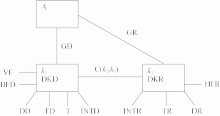 | Figure 1 Schematic diagram of rotational and divergent kinetic energy budgets in η coordinates. A represents the potential energy as shown in Fig. 1 of Buechler and Fuelberg (1986). |
The southwest vortex (SWV) in China often brings torrential rain events that result in catastrophic losses in lives and property. Because extrapolation of data to isobaric levels of the lower atmosphere contains inaccuracies, the actual structure and development of the vortex cannot be demonstrated in generally used weather maps. An eastward moving Tibetan Plateau vortex that later developed into an SWV and caused torrential rainfall was chosen as an example because it has been thoroughly analyzed by using isobaric datasets of higher levels ( He et al. , 2009). This vortex was generated from a closed depression cut off at more than 500 hPa near the Tibetan Plateau at 0800 UTC 20 July 2008, which continued to develop as it moved out of the Plateau at 1400 UTC 21 July 2008. Although the circulation at 500 hPa showed that divergent flow is important in maintaining the development of this vortex, the reanalysis data on isobaric surfaces failed to reveal its increasing intensity after movement out of the Plateau. Moreover, the sea level pressure, or surface pressure, obtained by National Centers for Environmental Prediction (NCEP) reanalysis data was determined to be similar to that observed in terrain studies and thus is used less frequently in direct analysis this vortex development ( Zhou et al. , 2012). Because energy budget analysis is an alternative method used to better understand the dynamics of weather systems, we performed comparative studies by using Eqs. (9) and (10) from the previous section to determine pressure and η coordinates.
NCEP reanalysis data recorded four times daily with a horizontal resolution of 1° × 1° and 26 isobaric levels were interpolated vertically onto 26 η layers. The integral approach for calculating stream function and velocity potential in a limited domain of arbitrary shape, developed by Xu et al. (2011), was used to obtain v2 and v3 in Eqs. (9) and (10).
Figures 2a and 2b illustrate the integrated kinetic energy for divergent wind ( K3) in pressure and η coordinates at 0800 UTC 21 July 2008, when this vortex moved away from the Plateau. Both figures show that the two maxi-mum centers were cut off by the Plateau, while the Fig. 2a corresponds to development of the SWV. Figure 2b shows stronger similarity in both pattern and amplitude than those in Fig. 2a; these parameters are not evident in the sea level pressure field (Fig. 5 in Zhou et al. , 2012).
Figures 3a and 3b present the temporal evolutions of vertical totals, from the model surface to the top, of the area-integration of K3 in pressure and η coordinates. K3 in η coordinates decreased in all cases, while DKD in Eq. (10) (Fig. 3d) became negative as soon as the vortex climbed the Plateau. We believe the increase in the first time interval shown in Fig. 3a may be attributed to the subsurface data beneath the Plateau.
Considering the advantages in η coordinates over pressure coordinates, Fig. 4 presents several budget terms of K3 in a vertical-temporal section to investigate the most influential term of this process. The terrain-related divergent term TD (Fig. 4b) exhibited maximum and minimum signals 6 h ahead of the emergence of the maximum in DKD at 0000 UTC 21 July, while the conversion term C( k2, k3) (Fig. 4c) appeared 12 h ahead. These results indicate that DKD was influenced faster by terrain effects than that by weather systems. Other terms (figures omitted) were negligible for this case.
This study aimed to explore the utilities of classic kinetic energy studies for rotational and divergent flows in mountainous areas. The new formulations in η coordinates, which are were based on previous studies of Buechler and Fuelberg (1986), explicitly show the terrain effects. A developing plateau vortex was diagnosed in both pressure and η coordinates as an example. Our major results are summarized in the following points:1) Kinetic energy studies provide an alternative method of obtaining dynamic information of the development of a vortex near a mountainous area when ordinary isobaric weather analysis fails.
2) Diagnostic and prognostic studies that use kinetic energy budget equations of rotational and divergent flow in η coordinates can avoid data voids, errors, and inconsistencies to provide more dynamic information on weather systems near mountainous areas. For the developing vortex case in this paper, applications of the previous budget equations in pressure coordinates are inaccurate due to unrealistic data at lower levels.
3) Although the kinetic energy analysis showed some potential advantages in η coordinates, limitations remain such that the physical explanations for v2 and v3 are not simply the rotational and divergent flow. Moreover, actual mountainous topography usually contains more intense small-scale structures, which constitutes a much more challenging test for the applicability and accuracy in interpolating reanalysis data fields. Such tests will be performed in our subsequent diagnostic studies with the help of datasets from local observatories. However, additional challenges may be introduced because inertia gravity waves need to be considered when analyzing sub-synoptic weather. These unaddressed and unresolved issues deserve further studies beyond this contribution.
To summarize, the kinetic energy budget equations for rotational and divergent flow formulated in η coordinates, shown in Eqs. (9) and (10), provide a new perspective for facilitating both diagnostic and prognostic studies for synoptic analyses in mountainous areas with model-simulated native datasets. Accurate numerical diagnoses can also be performed for other weather events in the Tibetan Plateau area from the perspective of kinetic energy studies; however, such studies are beyond the scope of this paper.
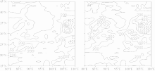 | Figure 2 Integrated kinetic energy for divergent wind in (a) pressure coordinates and (b) η coordinates at 0800 UTC 21 July 2008. |
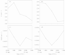 | Figure 3 Temporal evolutions of vertical totals, from model surface to top of the area integration of (a, b) K3 and (c, d) DKD in pressure and η coordinates from 0800 UTC 20 July to 1400 UTC 21 July 2008. |
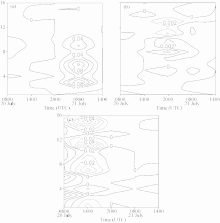 | Figure 4 Vertical-temporal sections of the horizontally integrated (a) DKD, (b) TD, and (c) C( k2, k3) over the area shown in Fig. 2 in η coordinates from 0800 UTC 20 July to 1400 UTC 21 July 2008, units in m2s-3. |
| 1 |
|
| 2 |
|
| 3 |
|
| 4 |
|
| 5 |
|
| 6 |
|
| 7 |
|
| 8 |
|
| 9 |
|
| 10 |
|
| 11 |
|
| 12 |
|
| 13 |
|
| 14 |
|
| 15 |
|
| 16 |
|
| 17 |
|
| 18 |
|
| 19 |
|
| 20 |
|
| 21 |
|
| 22 |
|
| 23 |
|
| 24 |
|
| 25 |
|
| 26 |
|
| 27 |
|
| 28 |
|
| 29 |
|
| 30 |
|