

The regional air quality modeling system RAMS-CMAQ (Regional Atmospheric Modeling System and Models-3 Community Multi-scale Air Quality) was developed by incorporating a vegetation photosynthesis and respiration module (VPRM) and used to simulate temporal-spatial variations in atmospheric CO2 concentrations in East Asia, with prescribed surface CO2 fluxes (i.e., fossil fuel emission, biomass burning, sea-air CO2 exchange, and terrestrial biosphere CO2 flux). Comparison of modeled CO2 mixing ratios with eight ground-based in-situ measurements demonstrated that the model was able to capture most observed CO2 temporal-spatial features. Simulated CO2 concentrations were generally in good agreement with observed concentrations. Results indicated that the accumulated impacts of anthropogenic emissions contributed more to increased CO2 concentra-tions in urban regions relative to remote locations. More-over, RAMS-CMAQ analysis demonstrates that surface CO2 concentrations in East Asia are strongly influenced by terrestrial ecosystems.
Projections of future atmospheric CO2 concentrations and associated climate forcing, and potential CO2 regulation, are primarily dependent on a scientifically sound understanding of the spatiotemporal distribution of atmospheric CO2 concentrations ( Peters et al., 2007). In 2007, the Intergovernmental Panel on Climate Change (IPCC) reported that anthropogenic emissions of CO2 substantially altered atmospheric composition ( IPCC, 2007). Oceans and terrestrial biosphere slow accumulation of CO2 in the atmosphere by absorbing approximately half of anthropogenic carbon emissions ( Hansen et al., 2007). Observations at surface stations in the northern hemisphere indicate that the seasonal cycle of atmospheric CO2 is driven primarily by net ecosystem production (NEP) fluxes from terrestrial ecosystems. Modern coupled atmosphere-biosphere models further suggest that terrestrial ecosystems, on a global scale, will provide a positive feedback in a warming world ( Heimann and Reichstein, 2008).
The spatiotemporal distribution of atmospheric CO2 concentrations in East Asia in recent years has been strongly influenced by biomass burning and urban and industrial activities. Previous attempts to assess time- space variability of CO2 concentrations have utilized global transport models ( Feng et al., 2011). However, the availability of high resolution sources and sinks enable scaling the spatiotemporal distribution of CO2 concentrations to a higher resolution within regional chemical transport models. The primary purpose of this study is to incorporate a vegetation photosynthesis and respiration module (VPRM) into the air quality modeling system RAMS-CMAQ (Regional Atmospheric Modeling System and Models-3 Community Multi-scale Air Quality) ( Zhang et al., 2002) to simulate CO2 concentrations. As far as we know, this is the first time that CMAQ has been applied to CO2 simulation. Given that transport is accurately represented, the modeling system can retrieve information on biospheric and anthropogenic controls of the source-sink distribution, at a greater spatiotemporal resolution than current global models. Furthermore, this coupled modeling system could deepen our understanding of the interaction between CO2 and atmospheric aerosols, as well as other gases, and enhance future studies on spatiotemporal patterns.
A short description of the modeling system, and its development to incorporate a VPRM module, are presented in section 2. In section 3, model results are evaluated against observations and discussed. Conclusions are given in section 4.
The model used in this study has two major components ( Zhang et al., 2002): RAMS ( Pielke et al., 1992) and Models-3 CMAQ ( Byun and Ching, 1999). CMAQ is an Eulerian-type model for concurrently simulating all atmospheric and land processes that affect the transport, transformation, and deposition of air pollutants and their precursors on both regional and urban scales. CO2 volume fraction is transported as a tracer in this model, with a prescribed surface CO2 flux that includes fossil fuel emission, biomass burning, sea-air CO2 exchange, and terrestrial biosphere CO2 flux.
The three-dimensional meteorological fields, required for CMAQ, are provided by RAMS. In this study, RAMS was excised in a four-dimensional data assimilation mode using analysis nudging with re-initialization every four days, leaving the first 24-h as the initialization period. The three-dimensional meteorological fields for RAMS were obtained from the National Centers for Environmental Prediction (NCEP) final analyses datasets (6-h intervals, 1° × 1° resolution). Weekly mean SST and observed monthly snow cover information provided the boundary conditions for RAMS calculations.
The study domain for CMAQ (shown in Fig. 1) was 6654 × 5440 km2 on a rotated polar stereographic map projection centered at (35.0°N, 116.0°E), with a grid resolution of 64 × 64 km2. This region has dramatic variations in topography and land types, entailing a mixture of industrial and urban centers and rural agricultural regions. RAMS and CMAQ have the same model height. For RAMS, there are 25 vertical layers in the σz-coordinate system, unequally spaced from the ground to ~23 km approximately nine layers of which are concentrated in the lowest 2 km of the atmosphere to resolve the planetary boundary layer. CMAQ uses 15 vertical levels, with the lowest seven layers being the same as those in RAMS.
The exchange of CO2 between the atmosphere and terrestrial biosphere is a central process in the carbon cycle and a critical determinant of Earth’s future state. The seasonal and spatial variation of biospheric CO2 flux is strongly influenced by the seasonal growth and decay of plants in terrestrial ecosystems. For example, biospheric CO2 flux is a carbon sink in Northern Hemisphere summer, as the uptake of atmospheric CO2 by photosynthesis exceeds CO2release by respiration in the growing season. While in winter, the biosphere acts as carbon source, since CO2 release by respiration exceeds uptake by photosynthesis. Generally, there are several approaches to simulate CO2 fluxes in vegetated areas, starting from highly simplified diagnostic models that use light and temperature sensitivity, derived from the eddy covariance observations ( Gerbig et al., 2003), and ending with sophisticated process-based ecophysiological models such as the simple biosphere modle (SiB2) ( Denning et al., 2003).
The terrestrial biosphere CO2 flux in CMAQ is calculated by incorporating a VPRM module. The approach to estimating biospheric CO2 flux was adopted from Gao et al. (2010) by assessing the net ecosystem production (NEP) from terrestrial ecosystems, the residual production from photosynthesis (i.e., Gross Primary Production, GPP) and the depletion from respiration ( R) fluxes. Unlike earlier VPRM, which used observed data each 16 days, the VPRM developed in this study specified for the diurnal variation of biospheric CO2flux by using hourly meteorological data from RAMS. The land cover information was provided by GlobCover satellite data, which has a horizontal resolution of 500 × 500 m2 and classifies the vegetation into 23 categories.
The VPRM calculated NEP on the principle of photosynthesis process and Light Utilization Efficiency (LUE), which demonstrated a linear relationship with GPP. GPP was calculated using: (1) LUE, which was a function of maximum solar energy utilization efficiency (vegetation type dependent: three majority types of vegetation were chosen at each grid), as well as water and temperature controlling factors (empirical theory); (2) Photosynthetically Active Radiation (PAR), provided by the total solar radiation (units: W m-2) that reaches earth’s surface from hourly averaged RAMS simulation; (3) Fraction of Photosynthetically Active Radiation (FPAR), calculated from the Enhanced Vegetation Index (EVI), which represents the fraction of shortwave radiation absorbed by leaves. In addition, VPRM accounted for the saturation of photosynthesis with increasing solar radiation. Respiration fluxes were calculated as a function of GPP and temperature based on the land cover conditions, obtained from Chinese Terrestrial Ecosystem Flux Research Network (ChinaFLUX) and the AmeriFLUX Network (AmeriFLUX) data. In this study, the land cover was divided into eight categories: broadleaf forest, coniferous forest, conifer and broadleaf mixed forest, farmland, grassland, wetlands, shrub, and soil. In our numerical experiments, the calculated NEP fluxes were provided to CMAQ as biospheric flux. Although the VPRM is a relative simple diagnostic model, it captures the temporal-spatial variations of biosphere-atmosphere fluxes remarkably well, and the limited number of parameters minimizes time- consuming calculation.
In addition to biospheric CO2 flux, the emission inventory also consisted of anthropogenic contributions, biomass burning and sea-air exchange. Ocean fluxes were obtained by the interpolation of global chemical transport models’ results. Anthropogenic emissions were adopted from the Regional Emission inventory in ASia (REAS, 2005 Asia monthly emission inventory) with a spatial resolution of 0.5° × 0.5° ( Ohara et al., 2007). Biomass burning emissions from forest wildfires, savanna burning and slash-and-burn agriculture were provided by Global Fire Emissions Database monthly mean inventory at a spatial resolution of 0.5° × 0.5° (Version 3, GFED v3) ( Van der Werf et al., 2010). Moreover, the initial fields of CO2 volume fraction, was obtained by interpolation of CarbonTracker results (data available at http://carbontracker.noaa.gov with global resolution of 3° longitude × 2° latitude).
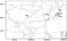 | Figure 1 Model domain and location of observation stations (Locations’ abbreviation listed in Table 1). |
The simulation period was from 1 January to 24 May 2007, starting at 0000 UTC 1 January. To assess the model’s ability to depict temporal-spatial features of CO2 concentration, modeled CO2 mixing ratios were compared with ground-based in-situ measurements from World Data Centre for Greenhouse Gases (WDCGG, http://ds.data.jma.go.jp/gmd/wdcgg/). The eight East Asia observation stations are located in Fig. 1, and their geographical information presented in Table 1. The performance of RAMS in diagnosing surface temperature and total solar radiation was also evaluated, to ensure precise meteorological input for CMAQ and VPRM.
The daily averaged surface temperature and total solar radiation between RAMS results and ground-based measurements are compared in Fig. 2. Observational surface temperatures were obtained from 728 Chinese stations and total solar radiation from 97 stations. As shown in Fig. 2, the simulated and observed surface temperature and total solar radiation were generally in good agreement (Figs. 2a-d). The correlation coefficients between observed and simulated temperatures were close to 1.0 (Fig. 2a), and were generally above 0.8 total solar radiation (Fig. 2d).
Time series data for simulated and observed CO2 concentrations at eight WDCGG stations are shown in Fig. 3. Observed CO2 values exhibited large variations in time and space. The model captured most observed temporal- spatial features reasonably well. The bias shown in Table 2 was less than 1.6% in most cases, indicating that the average model values were consistent with observations. Occasionally, the model performed less well in urban regions, e.g., in Fig. 3 at KIS and MKW, located in the urban regions of Japan. In urban regions it was difficult model for impacts of local emission fluctuations because input emission rates were based on monthly means. In addition, GSN was located at the western edge of the island with prevailing surface winds typically from the seaward direction. It was difficult for model with 64 km × 64 km resolution to capture the influence of such complex local topography and small scale system effects. In addition, the proximity to the eastern end of the Eurasia continent resulted in a strong influence of the Northern Hemisphere biogenic flux. In our study, the model could over-estimate the biospheric flux from photosynthesis and respiration of the terrestrial biosphere; a point for consideration and improvement in future studies.
As shown in Fig. 3, CO2 concentrations were generally higher at urban stations and lower at remote stations. The minimum observed mean value (386.6 ppm) appeared in the remote station WLG; while the maximum mean value (405.2 ppm) was reported in the urban station KIS. Remote stations with minimal human activity contributed less anthropogenic CO2 emissions; therefore, anthropogenic emission made greater contribution to increased CO2 concentrations in urban relative to remote regions. The variation in CO2 concentration in remote regions, with less human activity, was primarily influenced by the terrestrial ecosystem CO2 flux.
The horizontal distribution of simulated monthly average of CO2 concentrations and surface wind vectors are presented in Fig. 4. Greater monthly averaged CO2 concentrations above the ocean and lower values is in agreement with earlier studies ( Gangoiti et al., 2001; Zhang et al., 2002; Pérez-Landa et al., 2007). In the winter, a strong monsoon is predominant in East Asia due to large pressure gradients between the Siberian (Continental) High and Okhotsk (Maritime) Low. Typically, wind flow pattern indicates pollutant transport pathway. Thus, the dominant northward wind direction, due to this large scale weather pattern, is primarily responsible for pollutant transport from the Asian continent to the West Pacific region. In addition, less CO2 was absorbed by ocean than by lands, owing to greater photosynthetic uptake by terrestrial ecosystems, further contributing to higher atmospheric CO2 concentrations over the ocean.
The horizontal distribution of CO2 concentration from January to April is predominantly driven by the anthropogenic emissions and the variation in biospheric CO2 flux, arising from the seasonal growth and decay of land plants. As shown in Fig. 4, higher value areas of higher CO2concentration usually appear in the east and south of China, which often above 390 ppm concentration, with some regions reaching 400 ppm; while the northwest areas demonstrate lower CO2concentrations (380-390 ppm). This pattern of spatial distribution may primarily be attributed to local emissions; with southern regions highly industrialized areas where human activities contribute more CO2 emissions. Moreover, the relatively low concentrations in April in the east of China (about 380-390 ppm) demonstrated the influence of vegetation growth acting as a biospheric sink during this period (Fig. 4d). CO2 concentrations in East Asia, therefore, were strongly influenced by terrestrial ecosystem, as well as anthropogenic emissions.
| Table 1 Location of observation stations (NH, i.e., the Northern Hemisphere). |
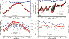 | Figure 2 Comparison of model results at the lowest model layer (~50 m above ground) (red dots) and observations at ground level (black lines): (a) averaged daily surface temperature (°C) and correlation coefficient (blue crosses) of the 728 observation stations; (b) yearly averaged surface temperature (°C) and correlation coefficient at each station; (c) averaged daily total solar radiation (MJ d-1) and correlation coefficient of 97 observation stations; (d) yearly averaged total solar radiation (MJ d-1) and correlation coefficient at each station. |
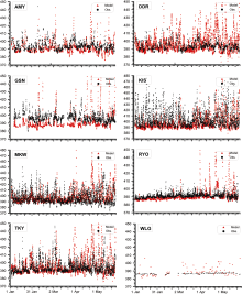 | Figure 3 Time series of simulated (red dots, units: ppm) CO2 mixing ratios at the lowest model layer (~ 50 m above the ground) and observed (black dots) hourly CO2 mixing ratios from 1 January to 24 May in 2007 at all stations, except daily averaged values are used for WLG. |
| Table 2 Statistical characteristics of simulated and observed CO2 concentrations at the observation sites, where Bias = 100% × (Simulated- Observed)/Observed. |
Coupled with a vegetation photosynthesis and respiration module ( Gao et al., 2010) accounting for the terrestrial ecosystem CO2 flux, the regional air quality modeling system RAMS-CMAQ was developed and applied to simulate the spatiotemporal distribution of atmospheric CO2 concentrations in East Asia. The CO2 volume fraction is transported as a tracer in this model with a pre- scribed surface CO2 flux that includes fossil fuel emis sions, biomass burning, sea-air CO2 exchange, and terrestrial biospheric CO2 flux. Comparison of model results with eight East Asia ground-based in-situ measurement stations from WDCGG indicates that the model reproduced temporal and spatial variations of CO2 concentrations reasonably well. The accumulated impacts of anthropogenic emissions play a more important role in the increase of CO2 concentrations in urban regions rather than remote regions. Further analysis of the horizontal distribution of CO2 concentration shows that the model correctly depicted physical processes, including transport and diffusion. In addition, the correlation between variation of CO2 concentration and biospheric CO2 flux suggests CO2 concentrations in East Asia are strongly influenced by terrestrial ecosystems. Finally, in order to simulate CO2 concentrations with high resolution, it is essential to use sources and sinks with precise details.
 | Figure 4 Monthly averaged horizontal distribution of atmospheric CO2 concentrations of 2007 (units: ppm) in (a) January, (b) February, (c) March, and (d) April. Also shown are surface-wind vectors (units: m s-1). |
This work was supported by the Strategic Priority Research Program-Climate Change: Carbon Budget and Relevant Issues (Grant No. XDA05040404) and the National Natural Science Foundation of China (Grant No. 41130528). We thank the WDCGG and all WDCGG data contributors for providing ground based CO2 measurements.
| 1 |
|
| 2 |
|
| 3 |
|
| 4 |
|
| 5 |
|
| 6 |
|
| 7 |
|
| 8 |
|
| 9 |
|
| 10 |
|
| 11 |
|
| 12 |
|
| 13 |
|
| 14 |
|
| 15 |
|