Climate simulations based on fluid dynamics encounter the problem of low-speed revolving fluid, which need long-time numerical integrations. Therefore, computational stability is very important for a numerical scheme to be used for solving the problem. For this reason, implicit and explicit schemes with exact square conservation have been developed successively, based on the physical integrals of geophysical motions, and applied successfully in numerical simulations of atmospheric and oceanic circulations ( Zeng and Ji, 1981; Ji and Zeng, 1982; Ji and Wang, 1991; Wang and Ji, 1993; Wang et al., 1993, 2004). However, these are all single-step conservative schemes and do not include historical observational data.

In order to incorporate historical observations, a variant of multistep schemes was constructed ( Chou, 1974; Cao, 1993; Cao and Feng, 2000). Taking into consideration the irreversibility of geophysical motions and utilizing effectively the information obtained from observational data, Cao (1993) formulated an appropriate difference-integral equation, called a self-memorization equation. He also proved that the existing multistep schemes can be unified in a framework of this self-memorization equation. However, these multistep schemes did not consider the computational stability and compatibility well; hence, they may encounter computational stability problems in a long-term integration.

All these led to the question whether we can construct a multistep scheme that not only conserves quadratic integral but also includes historical observations. This is an interesting topic and will be studied carefully in this paper.

First, we consider the evolution equation in an operator form:

, (1)

where F= F( x, t) is the undetermined function, x is the space variable, and t is the time variable. Suppose that the spatial differential operatoris antisymmetric, i.e.,. First of all, we discretizeusing the finite difference method, so that the spatial difference operator L compatible withalso becomes antisymmetric in the discrete space: ( LF, F)_d=0. In the following discussion, L is assumed to be a linear operator for the sake of simplicity.

We construct the ( k+1)-step finite difference scheme of Eq. (1) as follows:

(2)

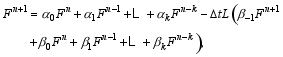
where α₀, α₁, L, α_k, β_-1, β₀, β₁, L, β_k are undetermined coefficients and denote this scheme as Scheme (2) (The following schemes we will use the similar representation). Here, they will be determined jointly by the requirements of compatibility and conservation and inclusion of historical observations.

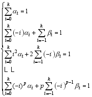
By means of the Taylor expansion, the local truncation error of Scheme (2) at t= t_n can be estimated. Scheme (2) becomes compatible with Eq. (1) with pth-order accuracy in time (where p< 2 k+ 2) when the coefficients α₀, α₁, L, α_k, β_-1, β₀, β₁, L, β_k satisfy the following conditions:

. (3)

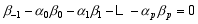
On the other hand, the generalized square conservation requires the coefficients in Scheme (2) to satisfy the following equation:

. (4)

Let us assume that p+ 1< 2 k + 2; this generates some free coefficients, which can be determined by fitting historical observations. In this way, all the coefficients can be determined, and a kind of generalized square conservative finite difference scheme that incorporates historical observations and is compatible with the original differential equation is constructed.

In the following, the two-step finite difference scheme is discussed in detail as an example of the new schemes.

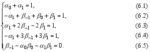
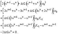
Setting k= 1 in Scheme (2), the two-step difference scheme is obtained:

. (5)

From Eqs. (3) and (4), the following equations of coefficients are deduced:

Solving Eqs. (6.1), (6.2), and (6.5), we get

.

Substituting this solution into Eq. (5), we derive an implicit two-step difference scheme that is stable and of first-order accuracy in time:

. (7)

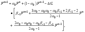
where α₀ and β_-1 remain as two free coefficients and can be estimated by fitting historical observations.

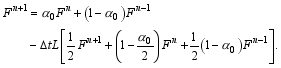
If β_-1=0, Scheme (7) becomes an explicit two-step scheme:

.(8) )

The remaining free coefficient α₀ can be estimated utilizing historical observations.

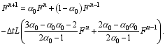
Setting α₀=0 and β_-1=1, separately, two second-order implicit two-step schemes are derived:

,

(9)

and

,(10)

The free coefficients in the above schemes are determined using historical observations.

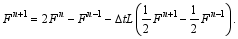
We can also construct some explicit and implicit two-step schemes without the inclusion of historical observations, such as the leapfrog scheme ( α₀= β_-1=0):

Fⁿ⁺¹= F^n-1- 2 LFⁿ. (11)

Similarly, the third-order implicit two-step scheme ( α₀=2, β_-1=1/2) is constructed:

(12)

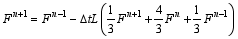
The fourth-order implicit two-step scheme (for α₀= 0, β_-1= 1/3) is as follows:

. (13)

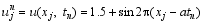
In order to examine the practicability of the new schemes, preliminary numerical tests are carried out based on the mixed problem of the one-dimensional linear advection equation:

,(14)

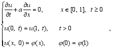
where u is the undetermined function, a is constant, and φ( x) is the initial function. The spatial differential operator, defined by, is antisymmetric under the periodic boundary condition u(0, t)= u(1, t). Setting φ( x) = 1.5 + sin2π x, the exact solution to Eq. (14) can easily be obtained, which is as follows:

. (15)

Here, central difference is applied to discretize, and a compatible spatial difference operator L is defined as follows:

, (16)

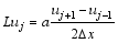
which also becomes antisymmetric in the discrete space under the periodical boundary condition shown in Eq. (14).

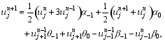
First, we discuss how the free coefficients of Scheme (7) can be determined by fitting historical observations. Because the operator L defined by Eq. (16) is linear, Scheme (7) can be rewritten in terms of α₀ and β_-1 as follows:

,(17)

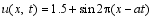
Historical observations are produced using exact solution (15):

,

where Mand N are constants. Substitute those values into Eq. (17), and then I (= NM) equations about α₀ and β_-1 are established and denoted simply by:

,(18)

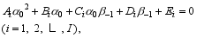
which can be solved by the nonlinear least-squares method and A_i, B_i, C_i, D_i, E_i are the simplified denotations of the corresponding parts in Eq. (17). Similarly, the free coefficients in Schemes (8)-(10) can be determined using historical observations.

Next, eight experiments with 10⁶ steps of integration are conducted using Scheme (7) (named “1st-im-beta- alpha”), Scheme (8) (“1st-ex-alpha”), Scheme (9) (“2nd- im-beta”), Scheme (10) (“2nd-im-alpha”), Leapfrog scheme (11) (“LF-2nd-ex”), Scheme (12) (“3rd-im”), Scheme (13) (“4th-im”), and the retrospective time integration ( Cao and Feng, 2000) (called the “Cao scheme”):

, (19)

whose coefficients α_-1, α₀, θ_-1, θ₀, β_-1, and β₀, are all determined by fitting historical observations, without considering compatibility and conservation. For all the experiments, set Δ x= 0.1, Δ t= 0.01, a= 1, and N = 32.

Finally, the performances of these schemes are evaluated, based on their root mean square errors (RMSEs), by comparing them with the exact solution and their conservations. The results show that, except for the Cao scheme that has a quick increase of RMSEs during the first 2300 steps of integration, all other schemes have their RMSEs within reasonable ranges (less than 0.6) (see Fig. 1). Among these schemes, Scheme (9) has the smallest RMSEs (less than 3×10^-3) after 10⁶ steps of integration; in contrast, RMSEs of the Cao scheme keep increasing and reach 10³ after 2800 steps of integration, although these are less than 5×10^-4 before 2000 steps of integration. In some tests in which N = 7, 23, 24, and 26, the Cao scheme has very small RMSEs (less than 5×10^-4) even after 10⁶ steps of integration, but in other cases (for N, 5-100), RMSEs of this scheme continue to increase till they become infinite before 3000 steps of integrations. It is indicated that the Cao scheme is not stable in terms of N. In contrast, the new schemes discussed in this paper remain stable for all cases of N from 5 to 100.

In terms of quadratic conservation (Table 1), in the Cao scheme, the total energy keeps increasing till it becomes infinite; on the other hand, two first-order schemes, Schemes (7) and (8), show a degression of energy during the early integration, but afterward energy remains constant at 22.5. Other five schemes conserve the energy well.

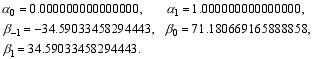
As a reference, the coefficients of Scheme (9) determined above ( N = 32) are shown here:

Figure 1

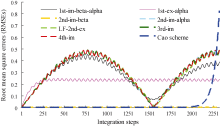Figure 1 RMSEs of eight schemes during 2320 steps of integration.

Generally, a scheme with energy conservation may have phase errors; this trend can clearly be observed in the results from four of the five schemes that conserve energy well (Fig. 2). The only exception is Scheme (9), which not only conserves energy well and keeps RMSEs small, but also has no phase error (Fig. 2). This is a surprising result. It suggests that proper consideration of accuracy, square conservation, and inclusion of historical observations is critical for the construction of a finite difference scheme.

Table 1

Table 1

Table 1 Evolutions of total energy of eight schemes. Step ( n) 1st-im-beta-alpha 1st-ex-alpha 2nd-im-beta 2nd-im-alpha LF-2nd-ex 3rd-im 4th-im Cao scheme 1 27.50000 27.50000 27.50000 27.50000 27.50000 27.50000 27.50000 27.50000 102 27.28259 23.45048 27.59956 27.51229 27.49972 27.51307 27.49892 27.5008 103 25.70228 22.50000 27.59495 27.50579 27.49893 27.49059 27.49816 27.5008 2.3 × 103 24.29404 22.50000 27.59357 27.50867 27.49994 27.52125 27.49893 61.1473 3 × 103 23.81323 22.50000 27.59487 27.50851 27.49957 27.48980 27.49820 1.9 × 1011 104 22.55799 22.50000 27.50042 27.50856 27.49934 27.52349 27.49922 Infinity 5 × 104 22.50000 22.50000 27.50229 27.50856 27.49999 27.53688 27.49898 Infinity 105 22.50000 22.50000 27.50499 27.50856 27.49994 27.47738 27.49824 Infinity 106 22.50000 22.50000 27.58304 27.50856 27.49829 27.47771 27.50001 Infinity

Table 1 Evolutions of total energy of eight schemes.

In this paper, a new method is proposed to construct finite difference schemes for evolution equations, whose coefficients are determined by prescribed accuracy, square conservation, and proper inclusion of historical observations. It is different not only from the traditional method of designing finite difference schemes that consider only accuracy and stability without the inclusion of historical observations, but also from the Cao scheme ( Cao and Feng, 2000) that fits only historical observations without considering compatibility and stability. Preliminary numerical tests based on the one-dimensional linear advection equation suggest that a finite difference scheme with reasonable consideration of accuracy, square conservation, and inclusion of historical observations may perform very well, with small RMSEs, good square conservation, and no phase error.

Because determination of the coefficients in the new schemes proposed in this paper involves only temporal As for the computing costs of the schemes, those with explicit solutions are time saving, thereby reducing costs, while those with implicit solutions are more expensive. In spite of its higher cost, implicit schemes may be suitable for the discretization in zonal direction to reduce the instability of a model in polar regions, as they generally have larger time steps.

discretization and is free from spatial discretization, it is not very difficult to apply these schemes to complex numerical models. A few coefficients determined through fitting historic observations or analysis/reanalysis data may actually play a role in the initialization or data assimilation to some extent. Implementation of the new schemes in real numerical models is similar to that in Eq. (14) and requires the spatial difference operator L, defined by Eq. (16), to be replaced by the spatial discrete operators of the models.

Figure 2

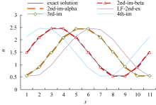Figure 2 Sine wave evolved after 106 steps of integration.