The Last Glacial Maximum (LGM, about 21000 calendar years ago) is a climate interval in which the global climate differed greatly from those of today, with lower atmospheric CO₂ concentration and more extensive ice sheets and sea ice, in addition to colder sea surface temperature (SST) (Jansen et al., 2007). The LGM has been a target period of the Paleoclimate Modelling Intercomparison Project (PMIP,Joussaume and Taylor, 1995); such simulations provide a good opportunity to examine model sensitivity to varying external forcing conditions and to evaluate their ability to simulate a climate different from the present. These are important for improving current climate models and providing a better understanding of past and present climate changes.

The ocean is an important component in the climate system and plays a key role in transporting meridional heat and moisture and in regulating large-scale atmospheric circulation. Therefore, the influences from various ocean surface conditions significantly affect the global climate, particularly in the monsoon areas (Ohgaito and Abe-Ouchi, 2009; Wang et al., 2010; Wang and Wang, 2013) and high-latitude areas (Braconnot et al., 2007; Jiang et al., 2012). In the first phase of the PMIP (PMIP1), numerous simulations were conducted by using atmospheric general circulation models (AGCMs) with prescribed SSTs derived from the Climate Long-Range Investigation, Mapping and Prediction (CLIMAP) project (CLIMAP, 1981). These model results generally simulated weaker global surface cooling during the LGM than that by reconstruction, which was attributed mainly to the weaker ocean surface cooling in the CLIMAP (Jansen et al., 2007). It was suggested that reliable depiction of LGM ocean surface conditions was crucial for more effective simulation of the LGM climate.

Within the second phase of the PMIP (PMIP2), seven ocean-atmosphere coupled general circulation models (OAGCMs) were used to simulate LGM climate. The dynamical ocean component indeed produced stronger SST cooling compared with the PMIP1 AGCMs. However, after the latest synthesis of LGM SST data was presented by the Multiproxy Approach for the Reconstruction of the Glacial Ocean Surface (MARGO) project (Waelbroeck et al., 2009), LGM tropical SST simulated by six PMIP2 OAGCMs was compared with the MARGO reconstructed LGM SST. It was revealed that most of the simulated LGM tropical SST cooling was greater than that observed by the reconstruction (Otto-Bliesner et al., 2009). A brief model-data comparison also suggested that some disagreement was apparent between the model and data in the North Atlantic (Waelbroeck et al., 2009). However, the interactive dynamical ocean in the PMIP2 OAGCMs has indeed contributed to better agreement in the model-data comparison (Braconnot et al., 2007).

Seven OAGCMs in the PMIP2 and five OAGCMs in the third phase of the PMIP (PMIP3) have been used thus far to simulate the LGM climate (Table 1), which has recently led to substantial development in the modeling community. Researchers have been inspired to determine whether the latest models show improvement in LGM SST simulation over the early OAGCMs in the PMIP2 and have examine the compatibility of the MARGO and OAGCM results in the North Atlantic, Tropical Ocean, and Southern Ocean, where data were plentiful. Conversely, little attention has been paid to model-model comparison in the PMIP2 and PMIP3 LGM SST simulations; these issues remain unclear and require further investigation. In this study, we used all of the available simulations under the framework of the PMIP to investigate the capability of the current models for simulating the LGM ocean surface conditions with particular attention on model-data and model-model comparisons.

The rest of this paper is organized as follows: Section 2 describes the PMIP LGM experimental design as well as models and data used in this study. Section 3 analyzes the simulated and reconstructed changes in SSTs during the LGM and offers a model-data comparison. Finally, concluding remarks are presented in Section 4.

The present study is based on all of the available simulations for the LGM within the PMIP, including seven OAGCMs simulations from PMIP2 and five OAGCMs simulations from PMIP3. For the LGM experiment, changes in boundary conditions include the Earth’ s orbital parameters, concentrations of atmospheric greenhouse gases, ice-sheet extent, and topography. The models were forced by an eccentricity of 0.018994, an obliquity of 22.949° , and a precession of 114.42° for the LGM simulations, which differs from the eccentricity of 0.016724, obliquity of 23.446° , and precession of 102.04° for the preindustrial (PI) simulations used as control experiments (Berger, 1978). Atmospheric CO₂, CH₄, and N₂O varied from the PI values of 280 ppm, 760 ppb, and 270 ppb, respectively, to 185 ppm, 350 ppb, and 200 ppb during the LGM period, respectively (Flü ckiger et al., 1999; Dä llenbach et al., 2000; Monnin et al., 2001). In the PMIP2, the ICE-5G ice-sheet reconstruction was used in the LGM experiments (Peltier, 2004). Conversely, the ice-sheet provided for the PMIP3 LGM experiments was a blended product obtained by averaging three different ice-sheet reconstructions including ICE-6G (Argus and

Peltier, 2010), GLAC-1 (Tarasov andPeltier, 2004), and Australian National University (ANU,Lambeck et al., 2010). Similar to that used for the reconstructed ice-sheet during the LGM, different values for land-sea mask, land surface elevation, and ocean bathymetry were used in the PMIP LGM experiments (Peltier, 2004; Argus and Peltier, 2010). Additionally, one of the PMIP3 OAGCMs, IPSL-CM5A-LR (see Table 1 for the full names of PMIP models), included carbon cycle in the LGM simulation. Additional details on the boundary conditions and experimental designs of the LGM simulations can be found at the websitehttp://pmip.lsce.ipsl.fr/.

Moreover, the reconstructed SSTs from the MARGO project were used to conduct the model-data comparison and to assess the capability of the current models for simulating SSTs during the LGM.

As illustrated in Fig. 1, PMIP models simulated global-scale ocean cooling during the LGM, which was caused mainly by lower greenhouse gas levels and a larger ice-sheet extent. Previous modeling studies (e.g.,Braconnot et al., 2007; Zheng and Yu, 2013), indicate that the lower concentrations of the atmospheric greenhouse gases could have resulted in a total decrease of approximately 2.8 W m^-2 in radiation forcing. As reported by Crucifix (2006), radiative forcing caused by the LGM ice-sheet varied from -7 W m^-2 to -14 W m^-2in annual mean depending on the model. However, these two negative forcings could have increased sea ice and led to positive feedback over the mid-and high-latitude ocean, which also may have contributed to the global cooling during the LGM. In this study, mid-latitude SSTs decreased by more than 4° C in both hemispheres compared with that observed in PI. The maximum cooling of -6° C was located over the mid-latitude northwestern Pacific and North Atlantic. Such significant tropical ocean cooling was also observed with the models, which was approximately 2° C lower than that observed with PI. Nevertheless, differences between these two generations of models remain. For example, PMIP3 OAGCMs simulated warm SST anomalies up to 2° C at southern Greenland over the North Atlantic, which differed significantly from the North Atlantic basin-scale cooling in the PMIP2 OAGCMs. Moreover, the PMIP3 OAGCMs produced stronger tropical cooling relative to the PMIP2 models. In addition, the standard deviation of simulated LGM SST among models was examined. The maximum standard deviation was observed over the North Pacific, North Atlantic, and mid-latitude Southern Ocean. These areas strongly correlated with the strongest ocean cooling, which implies large discrepancies for the simulated SST among the models. Compared with the PMIP2 OAGCMs, the PMIP3 OAGCMs simulated more consistent magnitude and patterns of ocean cooling at the LGM.

Table 1

Table 1

Table 1 Ocean-atmosphere coupled general circulation models (OAGCMs) within the PMIP2 and PMIP3 used in this study. Model Abbreviated name Oceanic resolution Project References 1. CCSM3.01 CCSM 1.125° × 0.27° , L40 PMIP2 Otto-Bliesner et al. (2006) 2. CNRM-CM332 CNRM-CM33 2° × 0.5° -2° , L31 PMIP2 Salas-Mé lia et al. (2005) 3. ECBILTCLIO3 ECBILTCLIO T63, L32 PMIP2 Vries and Weber (2005) 4. FGOALS-1.0g4 FGOALS 1° × 1° , L33 PMIP2 Yu et al. (2004) 5. HadCM3M25 HadCM3M2 1.25° × 1.25° , L20 PMIP2 Hewitt et al. (2003) 6. IPSL-CM4-V1-MR6 IPSL-CM4 2° × 2° , L31 PMIP2 Marti et al. (2005) 7. MIROC3.27 MIROC3.2 1.4° × 0.5° , L44 PMIP2 Hasumi and Emori (2004) 8. CNRM-CM58 CNRM-CM5 1° × 0.6° , L42 PMIP3 Voldoire et al. (2012) 9. GISS-E2-R9 GISS-E2 1.25° × 1, L32 PMIP3 Schmidt et al. (2006) Shindell et al. (2012) 10. IPSL-CM5A-LR10 IPSL-CM5A 2° × 1.2° , L31 PMIP3 Dufresne et al. (2012) 11. MPI-ESM-P11 MPI-ESM 1.4° × 0.8° , L40 PMIP3 Marsland et al. (2003) 12. MRI-CGCM312 MRI-CGCM3 1° × 0.5° , L51 PMIP3 Yukimoto et al. (2012) 1Community Climate System Model version 3; 2Centre National de Recherches Mé té orologiques Climate Model version 3; 3the atmospheric component ECBilt coupled to the free-surface ocean component CLIO; 4Flexible Global Ocean-Atmosphere-Land System Model, Grid-point Version 1.0; 5Hadley Centre Coupled Model, version 3; 6Institute Pierre Simon Laplace Coupled Model version 4-V1-MR; 7Model for Interdisciplinary Research on Climate version 3.2; 8Centre National de Recherches Mé té orologiques Climate Model version 5; 9Goddard Institute for Space Studies Model E version 2 with Russell Ocean Model; 10Institute Pierre Simon Laplace Coupled Model version 5A-LR; 11Max-Planck-Institute fü r Meteorologie Earth System Model; 12Meteorological Research Institute Global Atmosphere-Ocean Coupled Climate Model version 3.

Table 1 Ocean-atmosphere coupled general circulation models (OAGCMs) within the PMIP2 and PMIP3 used in this study.

The MARGO project has provided a more accurate picture of LGM SST by using a rigorous definition of the LGM time interval and multiproxy approach, relative to the CLIMAP project of the 1970s and 1980s. This latest reconstructed LGM SSTs provide an opportunity to evaluate model results, particularly those of the current models in the PMIP3. The MARGO compilation combines 696 individual SST reconstructions (Waelbroeck et al., 2009). The coverage is especially dense in the North Atlantic, Indian Ocean, Tropical Ocean, and Southern Ocean, but few records in the Pacific (Fig. 2a). The reconstructed LGM SSTs showed robust basin-scale cooling in the North Atlantic and Indian Ocean (Fig. 2b) with a maximum ocean cooling of 12° C in the mid-latitude North Atlantic. In addition, significant cooling was more pronounced in the eastern North Atlantic than that in the western North Atlantic, which extended into the Mediterranean. In contrast, positive SST anomalies were ob-served in the northwestern Pacific, tropical Pacific, and adjacent areas of the Greenland, the maximum of which was 4° C. Compared with the previous reconstruction by CLIMAP, however, the MARGO still depicted more extensive tropical cooling at the LGM.

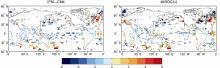
In this study, we focused on model-data comparison. As shown in Fig. 3, tropical cooling was more pro-nounced in most of the models than that in the MARGO reconstruction, with the exception of ECBILTCLIO, a PMIP2 OAGCM. Regarding the zonal average of the global ocean, the PMIP3 OAGCMs simulated stronger tropical cooling than that by the PMIP2 OAGCMs and MARGO reconstruction (Fig. 4a). For the North Atlantic, the MARGO gave a robust east-west SST anomaly gradient, indicating stronger-weaker cooling, which is considered a good target for evaluating model skill. All of the models, however, produced weaker cooling in the eastern North Atlantic and stronger cooling in the western North Atlantic, which is opposite the anomalous SST gradient present during the LGM. It appears that most of the current models are not able to capture the reconstructed LGM cooling features in the North Atlantic, which agrees with that reported byWaelbroeck et al. (2009). Additionally, the simulated SST anomalies in the North Atlantic differed significantly among the models (Fig. 4b), which implies large uncertainties in the simulated LGM North Atlantic SST.

Figure 1

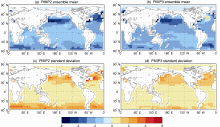Figure 1 Last Glacial Maximum (LGM) annual sea surface temperature (SST) anomalies simulated by Paleoclimate Modelling Intercomparison Project (PMIP) models and the standard deviation among the models (units: ° C) showing: (a) the ensemble mean of the second phase of the PMIP (PMIP2) ocean-atmosphere coupled general circulation models (OAGCMs), (b) the ensemble mean of the the third phase of the PMIP (PMIP3) OAGCMs, (c) the standard deviation of the simulated SST by the seven PMIP2 OAGCMs, and (d) the standard deviation of the simulated SST by the five PMIP3 OAGCMs.

Figure 2

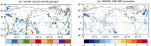Figure 2 Multiproxy Approach for the Reconstruction of the Glacial Ocean Surface (MARGO) proxy data showing: (a) number of proxy records per grid cell, and (b) MARGO-reconstructed LGM annual SST anomalies (units: ° C).

Figure 3

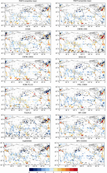Figure 3 Differences in simulated and reconstructed LGM annual SST anomalies calculated by subtracting MARGO results from those of the model (shaded area, units: ° C). Contours represent simulated LGM annual SST anomalies (units: ° C).

Figure 3

Figure 3 (continued)

The largest mismatch between the model and data was located in the northwestern Pacific. All of the models produced significant LGM cooling of 4° C-6° C in the northwestern Pacific. In contrast to the model results, a few MARGO records indicated LGM warming of 2° C or higher in the northwestern Pacific, whereas other records indicated LGM cooling of 0° C-4° C in that region. Therefore, the large mismatch between model and data was likely caused by the large uncertainties in the reconstructed data. Regarding the zonal average of the Pacific, most models simulated stronger cooling in the northern Pacific and weaker cooling in the southern Pacific than that observed with the MARGO (Fig. 4c). Moreover, the differences in simulated cooling magnitude in the mid-latitude southern Pacific showed larger discrepancies among the models. The MARGO and models both gave a more uniform distribution of LGM cooling in the Indian Ocean than that in the Atlantic and Pacific (Fig. 3). However, some discrepancies remained in the southern Indian Ocean among the models (Fig. 4d). On a basin scale, the ECBILTCLIO in the PMIP2 and the CNRM-CM5 in the PMIP3 simulated a weaker cooling in some areas of the Indian Ocean. Other models produced stronger LGM cooling than that given by the MARGO.

Figure 4

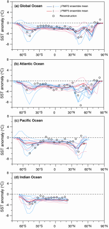Figure 4 Latitudinal averages of reconstructed and simulated LGM annual SST anomalies (units: ° C) for the (a) global ocean, (b) Atlantic Ocean, (c) Pacific Ocean, and (d) Indian Ocean. Circles represent MARGO-estimated LGM SST anomalies. Red and blue lines represent the ensemble mean of the LGM SST anomalies simulated by PMIP2 and PMIP3 OAGCMs, respectively. Pink and light blue lines represent PMIP2 and PMIP3 OAGCM-simulated LGM SST anomalies, respectively.

The outputs from twelve PMIP models were used to investigate changes in SST during the LGM. The model results suggested a tropical ocean cooling of 2° C and a mid-latitude ocean cooling of approximately 4° C in both hemispheres. Maximum cooling in excess of 6° C was observed in the northwestern Pacific and North Atlantic. In addition, larger standard deviations of the models were also presented over the stronger cooling areas, which implies larger discrepancies among the models, particularly in the Northwestern Pacific and mid-latitude North Atlantic. The PMIP3 OAGCMs showed a relatively small model-model mismatch compared with that given by the PMIP2 OAGCMs.

The model-data comparison indicated that most of the models in the PMIP simulated more pronounced tropical cooling than that given by the MARGO, with the exception of the ECBILTCLIO. For the North Atlantic, it was too difficult to identify whether OAGCM could simulate a similar eastern stronger cooling-western weaker cooling pattern as that suggested by the MARGO. All of the PMIP models simulated opposite changes in LGM SST in the northwestern Pacific, which includes warming in a few records and stronger cooling in the models. The large uncertainties in the data could explain the model-data mismatch in this case. Moreover, the current models still could not effectively capture the modern North Pacific SST variability reported in previous modeling studies (Zhang and Delworth, 2007; Furtado et al., 2011; Wang et al., 2012). This common problem in the models could have also contributed to the large model-data mismatch in the northwestern Pacific. In the Indian Ocean, the model-data mismatch was relatively small. Overall, this mismatch in the PMIP3 OAGCMs was smaller than that in the PMIP2 models, which was likely due to the higher resolution of the PMIP3 ocean models and the latest reconstruction of the LGM ice-sheet used in the PMIP3 experiments. However, the latest PMIP3 OAGCMs could not show substantial progresses in simulating the LGM SST. Therefore, improvements in both the modeling community and data are needed to more effectively explain LGM climate.