Accuracy and computational stability are two of the most important constraints in constructions of traditional finite difference schemes for both linear and nonlinear time-evolution partial differential equations. According to the undetermined coefficient method ( Wang and Ji, 2006), accuracy constraints can be easily applied for partly determining the coefficients of a finite difference scheme. However, applying the computational stability constraint in the construction of a difference scheme is quite complicated and difficult, particularly in designing difference schemes for nonlinear time-evolution equations. To deal with this difficulty, a stricter constraint for computational stability, quadratic conservation, is applied ( Zeng and Ji, 1981; Ji and Zeng, 1982). In general, square conservation in a difference scheme may keep its solution bounded in both the linear and nonlinear cases. It is easy to prove that in the linear case, boundedness of the solution is a necessary and sufficient condition of its computational stability. In the nonlinear case, however, it is very difficult to define computational stability like in the linear case. Therefore, Zeng and Ji (1981) defined the boundedness of the solution for nonlinear equations as their computational stability. In this way, maintaining square conservation in finite difference schemes is an important way to ensure their computational stability.

Early in the 1970s, Chou (1974) pointed out that including historical observations in a finite difference scheme would benefit its performance. However, no traditional finite difference schemes, including those with square conservation, used historical observations in their constructions. Following the thought of Chou (1974), a new class of multi-step finite difference schemes called retrospective time integration (RTI) schemes whose coefficients were determined by fitting historical observations were proposed ( Cao, 1993; Cao and Feng, 2000; Zhang et al, 2006; Gu et al, 2004). Numerical tests showed that this class performs well in a few cases when the number of observational samples is proper. However, they cannot maintain long-term computational stability in many other cases. Their computational stabilities seem very sensitive to the number of observational samples, and this becomes a bottleneck problem for further theoretical research and practical applications of RTI schemes ( Feng et al, 2004). The reason is that the determination of their coefficients did not use constraints for the compatibility or accuracy and computational stability or square conservation.

Can a finite difference scheme be constructed with an overall consideration of accuracy, square conservation, and information from historical observations? The answer is yes. Based on the undetermined coefficient method, Gong et al. (2013) constructed a kind of generalized square conservation scheme whose coefficients are partly determined by fitting historical observations in the linear case. Some of the new schemes show very good performance in the linear case. In the present paper, a three- step finite scheme constructed using the method in Gong et al. (2013) under the linear supposition will be generalized and applied to the solution of nonlinear time-evolution partial differential equations, and its performance in the nonlinear case will be discussed in detail with ideal numerical tests.

Consider a nonlinear time-evolution equation in operator form:

, (1)

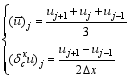
where F≡F(x, t) is the undetermined function, x is the space variable, and t is the time variable. The spatial differential operator in Eq. (1) is nonlinear, and anti-symmetrical, i.e., . It is easy to prove that Eq. (1) conserves the quadratic integral (or energy): . To keep this important conservation in the discrete scheme, the discretized operator of is based on a finite difference method, i.e., the spatial difference operator L, must satisfy two conditions: 1) it is compatible with , and 2) it is also anti-symmetrical in the discrete space: (LF, F)_d=0. In this way, the semi-discrete equation:

, (2)

also conserves the energy in the discrete space: .

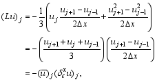
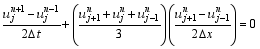
Now, it is the time to discretize the temporal differential term. Here we want to design a three-step finite difference scheme for solving Eq. (2), which is supposed to have the following form according to Gong et al (2013):

, (3)

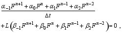
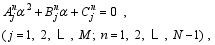
where α_-1, α₀, α₁, α₂, β_-1, β₀, β₁, and β₂ are undetermined coefficients and denote this scheme as Scheme (3) (The following schemes we will use the similar representation). The compatibility of Scheme (3) with Eq. (2) requires these coefficients to satisfy:

, (4)

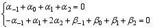
according to the Taylor expansion. A high-order approximation of Eq. (2) by Scheme (3) further asks the coefficients to obey:

, (5)

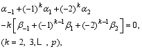
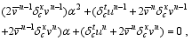
where p<6, so that there are some free coefficients left for the square conservation and fitting of historical observation. Note that for simplicity, Eqs. (4) and (5) are obtained under the linear supposition. Based on the anti-symmetry of L, it is easy to obtain the following equality from Scheme (3):

, (6)

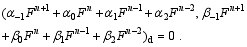
From Eq. (6), the necessary condition for the quadratic conservation of Scheme (3) is obtained as:

, (7)

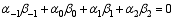
Now, there are ( p + 2) equations for the determination of eight coefficients, and there are (6 - p) free coefficients remaining. These free coefficients are used to fit historical observations to improve the performance of Scheme (3) further in long-term integrations.

In Eq. (5), p can be set to be 2-5, and then many schemes with different accuracy can be constructed. Because of the length limit for the present paper, we only choose the case as an example to show the determination of the coefficients in detail.

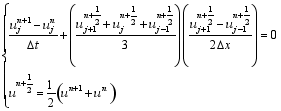
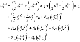
Set p=4 in Eq. (5) and solve Eqs. (4), (5), and (7) to obtain the following solutions:

, .

Substitute those solutions into Scheme (3). For simplicity, set α_-1=1 and α₀= α, where α is a free coefficient, then a three-step scheme, which has fourth-order accuracy in time, is obtained:

, (8)

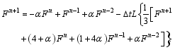
The free coefficient can be determined using historical observations.

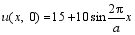
In order to examine the practicability of the new scheme, preliminary numerical tests are carried out based on the one-dimensional nonlinear advection equation:

, (9)

Set , t≥0, , and u(0, t) = u( a, t), where a= 6.3×10⁶ m, then Eq. (9) has the following implicit solution:

. (10)

To construct a scheme, the spatial differential operator is first discretized. In order to conserve the anti-symmetry in the corresponding spatial difference operator easily, a proper differential form is chosen for :

. (11)

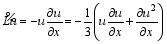
In this way, the spatial central difference can be directly employed to discretize the operator , and then a compatible spatial difference operator that naturally satisfies the anti-symmetry in the discrete space can be constructed as follows:

, (12)

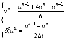
where

. (13)

In order to determine the free coefficient α of Scheme (8) by fitting historical observations, Scheme (8) is expressed as an equation of α:

, (14)

where

. (15)

Substituting the historical observations into Eq. (14), which are produced using the exact solution (10), gives:

,

,

where Mand N are constants. I (=( N?2)· M) equations about α are established:

, (16)

where N is the number of observational samples. The optimal solution to Eq. (16) can be obtained by the least-squares method.

For comparisons, three other schemes are given here based on Eq. (12), including the leapfrog (LF) scheme:

, (17)

the complete square conservative difference scheme (CSCD scheme) ( Zeng and Ji, 1981):

, (18)

and the retrospective time integration scheme (RTI scheme) ( Cao, 1993):

(19)

where α_-2, α_-1, α₀, β_-2, β_-1, β₀, θ_-2, θ_?1, and θ₀ are undetermined coefficients.

The LF scheme and CSCD scheme have no free coefficients. The RTI scheme has nine coefficients that are all determined by fitting historical observations without consideration of compatibility and conservation.

Set Δ x= 3×10⁴ m, and Δ t= 36 s. When the number of historical observation samples is 15, i.e., N = 15, the coefficient of the three-step scheme determined by Eq. (16) is

α= -0.499910278884411, while the coefficients of the RTI scheme in Eq. (19) are:

α_-2=-0.1707617115,

α_-1=0.4408313508,

α₀=0.9006921287,

β_-2=0.0052909003,

β_-1=-0.0104330067,

β₀=0.0050903851,

θ_-2=0.0015743143,

θ_-1=-0.0029990490,

θ₀=0.0013730159.

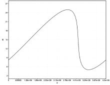
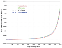
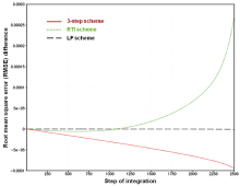
Because the schemes discussed above are not suitable for simulations of shock waves which require constructing special algorithms for their solutions, all comparisons between these schemes will be at the time before the 2500th step of integration when shock waves do not occur in the exact solution, although a large gradient begins to appear at this step (Fig. 1). The three-step scheme, RTI scheme, LF scheme, and CSCD scheme all perform quite well during this period, with small root mean square errors (RMSEs), compared with the exact solution (Fig. 2). However, the best performance of the three-step scheme and worst performance of the RTI scheme can be clearly seen in Fig. 2. To make the differences in their performances clearer, a reference is subtracted from their RMSEs, which is chosen as the RMSE of the CSCD scheme (Fig. 3). It is clearly observed from Fig. 3 that the three-step scheme produces increasingly smaller RMSEs compared to the CSCD scheme over time, while the RTI scheme produces increasingly larger RMSEs. The LF scheme has RMSEs very close to those of CSCD scheme, as can be seen in both Figs. 2 and 3. Further, using the differences of the RMSEs between the three-step scheme and the other three schemes to be divided by the RMSEs of the other three schemes, respectively, the percentages decreases of RMSE in the three-step scheme relative to the other three schemes are obtained (Table 1). The decrease of the RMSEs in the three-step scheme are obvious, par ticularly in the early period of integration. It is easy to understand that the three-step scheme benefits from the overall consideration of compatibility, square conservation, and fitting to historical observations to achieve the best accuracy, while the largest RMSEs of the RTI scheme after 1000 steps of integration can be attributed to the absence of the compatibility and square conservation constraints, although this scheme outperforms the LF scheme and CSCD scheme in the first 1000 steps due to its inclusion of historical observations.

Figure 1

	Figure Option ViewDownloadNew Window
	Figure 1 Exact solution of Eq. (9) at the 2500th step.

Figure 2

	Figure Option ViewDownloadNew Window
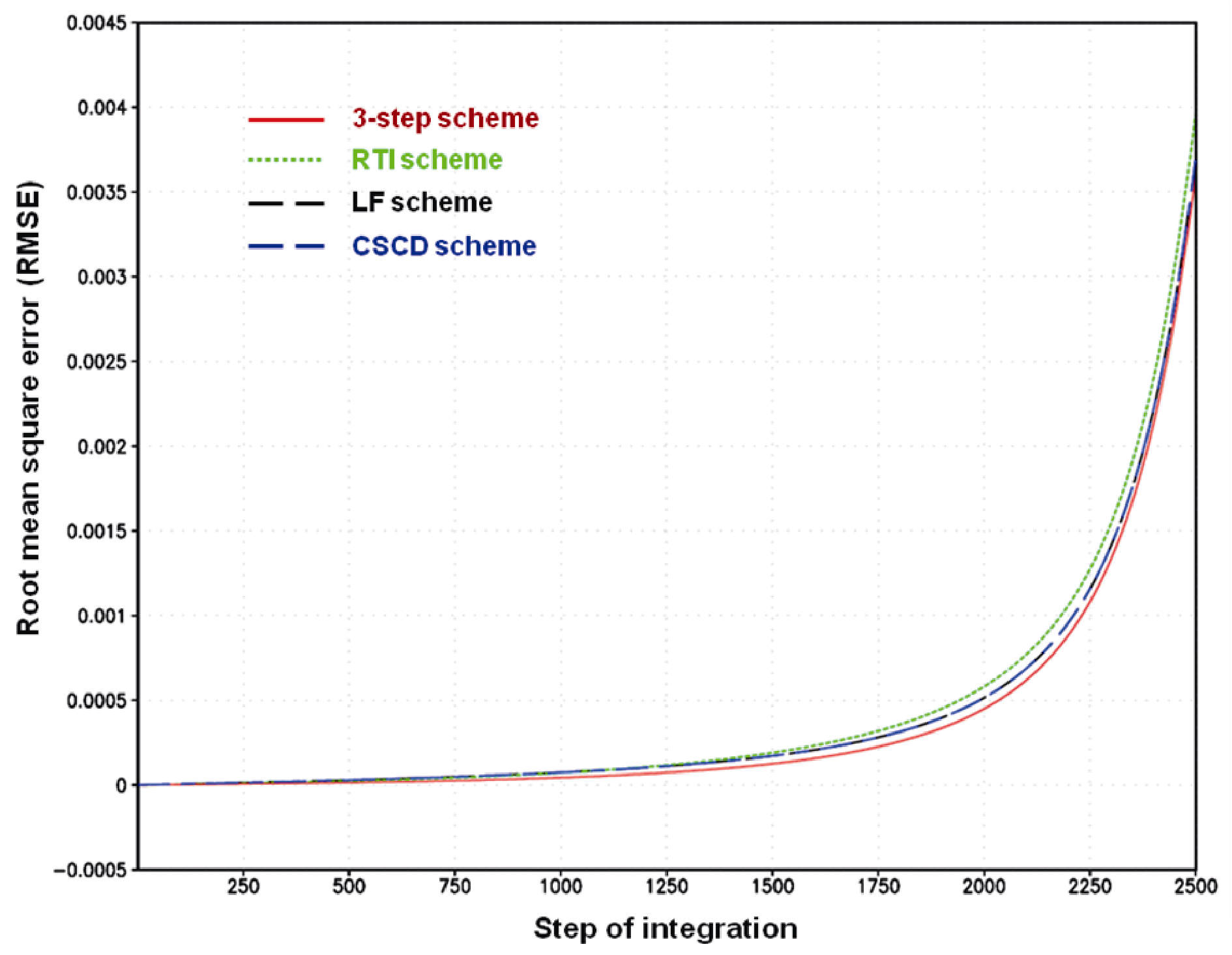	Figure 2 RMSEs of four schemes from 1 to 2500 steps of integration.

Figure 3

	Figure Option ViewDownloadNew Window
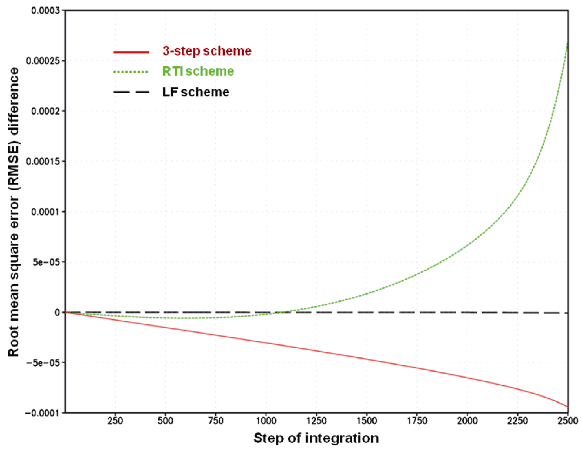	Figure 3 Difference of RMSEs between the three schemes and the CSCD scheme.

Table 1

Table 1

Table 1 Percentages of RMSE decreases in the three-step scheme relative to the other three schemes (%). Steps LF scheme RTI scheme CSCD scheme 100 55.1745 37.7602 55.3464 1000 40.8611 39.3663 40.9233 1500 26.9804 34.0469 27.0207 2000 12.5719 22.5795 12.6048 2500 2.5167 9.1291 2.5349

Table 1 Percentages of RMSE decreases in the three-step scheme relative to the other three schemes (%).

The lack of compatibility and square conservation in the RTI scheme also leads it to be very sensitive to the number of historical observation samples (Table 2). It is computationally unstable unless N = 15 (Table 2). However, the newly proposed three-step scheme remains stable for any N due to the constraints of compatibility and square conservation.

This suggests that overall consideration of accuracy, square conservation, and incorporation of historical observation in constructing a finite difference scheme is very important for it performance.

In the present paper, a new three-step finite difference scheme for nonlinear time-evolution partial differential equations was proposed. Compared to the undetermined coefficient method, the coefficients of the new scheme are partly determined based on its compatibility and the necessary condition of square conservation, similar to the construction strategy of traditional difference schemes. Meanwhile, the free coefficients of the scheme left are further determined by fitting historical observations according to the approach of Cao (1993). Because the new scheme includes the advantages of both traditional differences (e.g., the LF scheme and CSCD scheme) and the RTI scheme, it outperforms all of them in numerical experiments conducted using the one-dimensional nonlinear advection equation. The results of the experiments suggest that overall use of accuracy constraints, the necessary condition of square conservation, and incorporation of historical observations are very important for the con struction of finite difference schemes and may benefit their performance.

Table 2

Table 2

Table 2 RMSEs at the 2500th step of integration. The number of historical observation samples N = 5 N = 15 N = 30 N = 60 N = 150 RMSEs of RTI scheme infinite 4.000199×10-3 infinite infinite cannot run RMSEs of three-step scheme (×10-3) 3.635017 3.635014 3. 635006 3.634976 3.634775

Table 2 RMSEs at the 2500th step of integration.

As in the linear case, the new three-step scheme proposed in the present paper is easy to apply to complex numerical models. As for its computing cost, the scheme is more expensive because of its implicit solution. However, it can use larger time step sizes to reduce computing costs. Therefore, it will hopefully be applied to real numerical models.