A Local Implementation of the POD-Based Ensemble 4DVar withR -Localization
Cite this Article
TIAN Xiang-Jun. A Local Implementation of the POD-Based Ensemble 4DVar withR -Localization . Atmospheric and Oceanic Science Letters, 2014, 7(1): 11-16 
Permissions
Copyright?2014, Editorial office of Atmospheric and Oceanic Science Letters
This is an Open Access article under the terms of CCAL.
A Local Implementation of the POD-Based Ensemble 4DVar withR -Localization
Abstract
The purpose of this paper is to provide a robust and flexible implementation of a proper orthogonal decomposition-based ensemble four-dimensional variational assimilation method (PODEn4DVar) through
Keyword:
PODEn4DVar; R-localization; local implementation
1 Introduction
The ensemble Kalman filter ( EnKF, Evensen, 1994, 2004; Houtekamer and Mitchell, 1998, 2001; Hamill et al., 2001) provides an advanced alternative solution to data assimilation in various weather ( Snyder and Zhang, 2003; Tong and Xue, 2005; Chen and Snyder, 2007; Meng and Zhang, 2008; Wang et al., 2008; Whitaker et al., 2008; Aksoy et al ., 2009; Dowell and Wicker, 2009; Torn and Hakim, 2009; Bonavita et al., 2010; Miyoshi et al., 2010) and climate applications ( Whitaker et al., 2004; Compo et al., 2011). Besides its simple conceptual formulation and relative ease of implementation, EnKF has the ability to evolve flow-dependent estimates of forecast error covariance by forecasting the statistical characteristics. However, the EnKF does not include the temporal smoothness constraint assumed in the standard four-dimensional variational assimilation method ( 4DVar, e.g., Lewis and Derber, 1985; Le Dimet and Talagrand, 1986; Courtier and Talagrand, 1987; Courtier et al., 1994) because its design concept incorporates observational information sequentially. Thus, significant efforts have been devoted to enhance data assimilation by coupling 4DVar with EnKF to combine their strengths (e.g., Lorenc, 2003; Qiu et al., 2007; Tian et al., 2008, 2011; Tian and Xie, 2012; Zhang et al., 2009; Cheng et al., 2010; Wang et al., 2010). The proper orthogonal decomposition (POD)-based ensemble four-dimensional variational assimilation method (referred to as PODEn4DVar; Tian et al., 2008, 2011; Tian and Xie, 2012) is proposed based on POD and ensemble forecasting techniques. In the PODEn4DVar, the original ensemble coordinate system is transformed into an optimal scheme under the usual Euclidean norm ( Ly and Tran, 2001) through the POD process, which improves assimilation performance. Its feasibility and effectiveness have been demonstrated through the use of an idealized model with simulated observations ( Tian et al., 2011; Tian and Xie, 2012) and the Weather Research and Forecasting (WRF) model with real radar data ( Pan et al., 2012). Moreover, PODEn4DVar also provides a promising method for land data assimilation ( Tian et al., 2009, 2010).
In ensemble data assimilation, localization is generally adopted to ameliorate the spurious correlations of observations from distant regions that occur in analyses (e.g., Houtekamer and Mitchell, 2001; Hamill et al., 2001), thus providing better results in many cases (e.g., Greybush et al., 2011; Miyoshi et al., 2010; Szunyogh et al., 2008). Additionally, analysis at each grid point can be implemented independently with only local observations and the values at nearby model grid points needing consideration; thus, more efficient parallelization of the code can be realized ( Hunt et al., 2007; Szunyogh et al., 2008; Greybush et al., 2011).
As discussed by Greybush et al. (2011), two classes of localization techniques in general usage include B-localization and R-localization. The former operate on background error covariances B, while the latter are those that modify observation error covariances R. Although it has been developed mainly in the EnKF community, the localization technique is also indispensable in ensemble-based variational assimilation methods (e.g., Tian et al., 2008, 2011; Tian and Xie, 2012; Wang et al., 2010). The PODEn4DVar uses a variation of B-localization, in which there is no direct modification on the observation error covariance R ( Tian et al., 2011; Tian and Xie, 2012). Unfortunately, previous studies note that both types of localization can disrupt the relationships and thus result in unrealistic imbalances between mass and wind fields in analysis ensembles (e.g., Kepert, 2009; Greybush et al., 2011). Because the B-localization scheme is more prone to imbalance and greater errors in analysis and forecasting, implementation of R-localization in PODEn4DVar has the potential for improving assimilation performance.
The main purpose of this paper is to describe a local implementation for PODEn4DVar through the R-localization scheme with emphasis on facilitating its parallel coding with improved assimilation performance. The rest of the paper is organized as follows. In section 2, we describe the local implementation for PODEn4DVar with R- and B-localization schemes after a simple review of PODEn4DVar. In section 3, observing system simulation experiments (OSSEs) are conducted with no localization and with R- and B-localization schemes for evaluation of PODEn4DVar. Finally, a summary is given in Section 4.
2 Local implementation for PODEn4DVar through R-localization
2.1 Review of PODEn4DVar
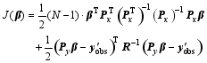
The incremental format of the 4DVar cost function is formulated as
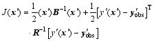 | , (1) |
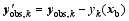
where x′ = x- xbis the perturbation of the background field xbat the initial time t0,
 | , (2) |
 | , (3) |
 | , (4) |
 | , (5) |
 | , (6) |
and
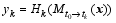
Here, the superscript T represents a transpose, b denotes background value, index k stands for observation time, Sis the total observational time steps in the assimilation window, Hk acts as the observation operator, and matrices B and Rk are the background and observational error covariances, respectively. In this study, Rk is assumed to be diagonal. The 4DVar cost Eq. (1) should be minimized to obtain an optimal increment of initial condition (IC), x′a, at t0, where the subscript a denotes an optimal value, obs denotes the observational values.
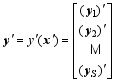
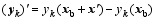
In PODEn4DVar ( Tian et al., 2011), an ensemble of Nobservation perturbations (OPs) y′: 


( y′)T y′ = V?2 VT, (8)
Py = y′ V, (9)
and
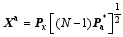
Px = x′ V, (10)
where V is an orthogonal matrix, ?is a diagonal matrix, Px and Py are the POD-transformed MP and OP matrixes, respectively.
The optimal solution x′a and its corresponding optimal OP y′ais thus expressed by linear combinations of the POD-transformed MPs and OPs, respectively, as
x′a= Pxβ, (11)
and
y′a= Pyβ, (12)
where β is the coefficient vector.
Substituting Eqs. (11) and (12) and the ensemble background covariance 
Through simple calculations reported by Tian et al. (2011), the solution to the increment of analysis is simplified into the following form:
 | , (14a) |
where I is the unit matrix.
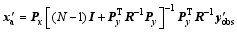
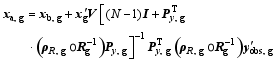
Substituting Eq. (10) into Eq. (14a), the expression can be modified as
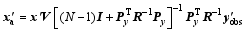
The final PODEn4DVar analysis without localization is easily obtained as
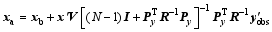
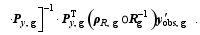
Obviously, Eq. (15a) can be implemented independently for each [ ith, 1≤ I≤dim( xb)] grid point as
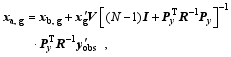 | (15b) |
where x′g, xb, g, and xa, g represent MPs, background, and analysis states for each ( ith) grid point, respectively.
Conversely, the analysis ensemble perturbation matrix is updated through
 | , (16) |
where 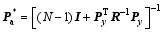
2.2 Local implementation for PODEn4DVar
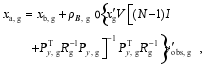
It is reasonable to assume that R is diagonal with uncorrelated observation errors. Hunt et al. (2007) proposed a gradual R localization by multiplying the diagonal elements of R by an increasing function ρR of distance from the analysis grid point. Because PODEn4DVar shares similar formulations with the local ensemble transform Kalman filter ( LETKF; Hunt et al., 2007), we can easily implement the R-localization scheme into the final PODEn4DVar analysis as
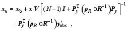 | (17) |
where 
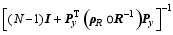


 | , (18) |
where ρR, g is the local localization matrix, y′obs, g is the local innovation vector, Rg is the local observational error covariance, and Py, g is the local POD-transformed OP matrix.
The local vectors and matrices (i.e., y′obs, g, Rg, ρR, g, and Py, g) can be formed under the following conditions:(a) dim( y′obs, g) = 0;(b) For any 1≤ j≤dim( y′obs, g), compute ρR, g, j;(c) If ρR, g, j > ε (where ε> 0 is a small preset parameter), dim( y′obs, g) = dim( y′obs, g)+1; store j in a preset integer vector dim Loc;(d) All the ρR, g, j > ε constitute the local localization matrix, ρR, g;(e) s = dim Loc( j) [1≤ j≤dim( y′obs,g)]; extract all ( sth) elements of y′obs, the ( sth) diagonal elements of R, and the ( sth) rows of Py to construct the local innovation vector y′obs, g, the local observational error covariance Rg, and the local POD-transformed OP matrix Py, g, correspondingly.
Therefore, the local implementation of PODEn4DVar requires the following steps:1) Run the forecast model repeatedly ( N times) to obtain an ensemble of Nobservation perturbations (OPs) y′ by using the observation operator Hk and the MPs x′;2) ( y′)T y′ = V?2 VT;3) Py = y′ V;4) Form y′obs, g, Rg, ρR, g, and Py, g under the conditions of (a)-(e);5) 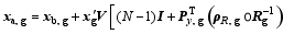
Apparently, the dimensions of the local observational matrices and vectors are substantially lower than the original values because numerous computational resources are thus released. In addition, the implementation of the local analysis steps 1) - 5) is apt to be coded in parallelization.
As mentioned in the Introduction, the original version of PODEn4DVar uses a variation of B-localization ( Tian et al., 2011; Tian and Xie, 2012):
 | (19) |
which can be also implemented locally as
 | (20) |
where ρB, g is the local covariance localization matrix.
3 Evaluations within a shallow-water equation model
3.1 Design of OSSEs
To examine the performance of PODEn4DVar with R-localization in comparison with the original version of the method with B-localization and that without localization, it is convenient to design OSSEs by using the same shallow-water equation model with the same parameter settings as that reported by Tian and Xie (2012). Particularly, the model domain is square with 45 
 | , (21) |
with the maximum height set to h0= 250 m for the true model and h0= 0 m for the imperfect model.
The initial condition and initial ensemble were generated in the same manner as that described by Tian and Xie (2012). Accordingly, the observation errors were assumed to be uncorrelated between different variables and different points in space and time. Simulated observations were generated every 3 h by adding random errors to the model-produced true fields at sparsely selected grids spaced every 3 d = 900 km in the x- and y-directions. The observation error standard deviations were set to 1.5 m for h and 0.21 m s-1 for u and v. In all assimilation experiments, the weighting covariance inflation technique proposed by Zhang et al. (2004) was used to relax or weight the previous and updated ensembles; the relaxation coefficient was set to 

3.2 Experimental results
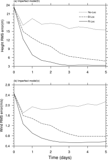
A group of experiments in the presence of model error with a maximum terrain height of h0= 0 m in the forecast model was conducted to investigate the performance levels of all three PODEn4DVar schemes including B-localization, R-localization, and no localization. Truth simulations ( h0= 250 m) were used for verification and for generating observations. Figures 1a and 1b compare the performances of the three schemes under the imperfect model assumption ( h0= 0 m). Remarkably, under the imperfect model scenario, the superior performance of the R-localization over the other two schemes was obvious from the beginning of the second assimilation window through the end of the entire assimilation process. Such a conclusion is also strongly supported by the special error statistics over the last assimilation window such that the spatial mean root-mean-square (RMS) error produced by the R-localization scheme was smallest at 3.31 m and 0.57 m s-1for height and wind fields, respectively. Correspondingly, the spatial RMS errors produced by the B-localization scheme were 4.79 m and 0.78 m s-1 for height and wind, respectively. No convergent solution was obtained by the no-localization case.
 | Figure 1 Spatially averaged (a) height root-mean-square (RMS) errors and (b) wind RMS errors for the proper orthogonal decomposition -based ensemble four-dimensional variational assimilation method (PODEn4DVar) under the imperfect model scenario ( h0= 0 m). Schemes without localization and with B- and R-localization are represented by dotted, dashed, and black solid lines, respectively. |
The computational costs for PODEn4DVar with various localization schemes, including no-localization and serial coding, were compared through the central processing unit (CPU) time (units: s) required to complete their respective assimilation experiments. As shown in Table 1, R-Loc-g denotes the R-localization scheme (i.e., Eq. (18)), B-Loc-g represents the B-localization scheme (i.e., Eq. (20)), No-Loc stands for PODEn4DVar implementation without localization Eq. (15a), and No-Loc-g represents no localization but independent implementation for each grid point (i.e., Eq. (15b)). The No-Loc case showed the lowest total CPU time at 345.6 s because repeated computation of the term 
It should be noted that an additional group of experiments under the perfect-model scenario was conducted, and results similar to those of imperfect model case in this study were obtained (not shown). Moreover, the sensitivity of PODEn4DVar with R-localization to parameters such as ensemble size, inflation, and others reported by Tian and Xie (2012) has also been tested.
| Table 1 Central processing unit (CPU) time for the PODEn4DVar with various localization schemes. |
5 Summary and concluding remarks
This study has upgraded the POD-based ensemble 4DVar method through a local implementation with R- localization. The R-localization scheme is first introduced to the PODEn4DVar analysis formula, which is followed by a step-by-step description of its efficient local implementation. Local implementation of the original version of PODEn4DVar with B-localization is also presented. For comparison, PODEn4DVar without localization, implemented locally in the same manner as that of localization schemes, is also discussed. The robustness and potential merits of the local implementation of PODEn4DVar with R-localization are demonstrated through OSSEs by using a two-dimensional shallow water model. The local implementation of PODEn4DVar with no localization and B-localization are also adopted to fulfill the same OSSE conditions. The assimilation results imply that the local PODEn4DVar with R-localization outperforms the original version with B-localization to a certain extent, particularly under the imperfect model scenario. An analysis of the computational costs demonstrates that PODEn4DVar local implementation with R-localization is significantly more efficient than the other schemes due to its easy parallelization.
Reference
| 1 |
|
| 2 |
|
| 3 |
|
| 4 |
|
| 5 |
|
| 6 |
|
| 7 |
|
| 8 |
|
| 9 |
|
| 10 |
|
| 11 |
|
| 12 |
|
| 13 |
|
| 14 |
|
| 15 |
|
| 16 |
|
| 17 |
|
| 18 |
|
| 19 |
|
| 20 |
|
| 21 |
|
| 22 |
|
| 23 |
|
| 24 |
|
| 25 |
|
| 26 |
|
| 27 |
|
| 28 |
|
| 29 |
|
| 30 |
|
| 31 |
|
| 32 |
|
| 33 |
|
| 34 |
|
| 35 |
|
| 36 |
|
| 37 |
|
| 38 |
|
| 39 |
|
| 40 |
|