Wind power, as an alternative clean energy source to fossil fuels, supports environmental sustainability and possibly provides part of the solution to our energy security problem ( Pryor and Barthelmie, 2011). The wind energy resource in the atmospheric boundary layer has been investigated in detail in many countries ( Bryukhan and Diab, 1995). Increasing the value of wind generation through the improvement of the performance of prediction systems is one of the priorities for wind energy research in the coming years ( Karimiotakis et al., 2004). One of the necessary conditions for the development of wind power generation is to choose the optimal site. Objective and accurate wind resource assessment is vital, and plays an important role in promoting large-scale wind farms. Currently, the methods of wind energy assessment from other countries are mainly based on traditional data observation or evaluation and numerical simulation. The methods based on long-term observations are comparatively expensive in operation and initial costs, so they are much more sparsely deployed. With the increasing number of wind turbines, an additional observational source has become available: quasi-routine observations at the top of the nacelle of some of the wind turbines. Although these measurements are downwind of the rotor blades, they can provide valuable information on the wind energy layer ( Drechsel et al., 2012). Therefore, while the most common approach is to build an anemometer tower in the location of the wind farm, the application of numerical weather prediction (NWP) models for the simulation of wind conditions in a given area is another important method. Mesoscale NWP model predictions are integral to the forecast process ( Ma et al., 2009).

Wind is an important forcing factor of the coastal oceans ( Allen, 1980). Xincheng, located in the southwest of Liaoning Province—an area where the wind has a strong influence—is home to a coastal wind farm (specific location: 40°21.808'N, 120°34.148'E). The measurement sites here encompass a variety of terrain: offshore, coastal, flat, hilly, and mountainous regions, with low and high vegetation, and also urban influences. The surrounding terrain of the wind farm is very flat, and close to the coast. The strongly differing site characteristics modulate the relative contribution of synoptic-scale and smaller-scale forcings to local wind conditions, and thus the performance of the NWP model ( Drechsel et al., 2012). In this paper, we report results of an assessment of the wind energy at the Liaoning coastal wind farm using observational data and NWP model forecast time series at observation locations over two years. The differences between the observed and simulated results were analyzed to see whether the Weather Research and Forecasting (WRF) model is able to reliably assess the wind power resource of this location.

Relatively complete and continuous observational data were used to verify whether the WRF model can assess the wind power density accurately, as continuous self- recording wind speed is helpful in improving the accuracy of wind energy assessment. Increasing scientific and public interest in the assessment of wind resources means that high temporal resolution observations are required, and ultimately that fully-functioning wind farms and wind turbine parameters are available and of benefit to the public. Nevertheless, difficulties exist insofar as wind measurements are generally performed below wind turbine hub heights because of the lower measurement and mast costs ( Đurišić and Mikulović, 2012). Furthermore, most wind farms are not located within synoptic weather observational networks, which makes the use of conventional meteorological data challenging ( Zhou et al., 2013). However, in this study, wind speed and wind direction data at 10-minute intervals and average continuous observations at a height of 70 m were used from 1 January 2009 to 31 December 2010. Therefore, spatial and vertical extrapolations of measured data were not needed. Apart from some missing data, there were 144 time series in a day, and all times used in this report were local times that were then changed to UTC.

To assess the wind power density using the WRF model through dynamical downscaling, we used National Centers for Environmental Prediction (NCEP) Final (FNL) Operational Global Analysis data to verify the results. These data are available on 0.5°×0.5° grids prepared operationally every six hours. The analyses are available at the surface, at 26 mandatory levels from 1000 hPa to 10 hPa, in the surface boundary layer, and at some sigma layers, in the tropopause, among others.

The WRF model is a numerical weather prediction system for both research and operational forecasting purposes. The WRF model parameters are often used to represent the interaction between different scales in the process of model calculation. Using microphysics, shortwave radiation and atmospheric longwave radiation, cumulus parameterization, boundary layer, and a physical parameterization scheme, the WRF model improves simulation results. In this study, the model used NCEP global 30-s topographic data and NCEP/NCAR (National Center for Atmospheric Research) reanalysis data as initial and lateral boundary conditions. Details of the FNL reanalysis data used were described above.

Figure 1 shows that there were three nested domains under consideration, and the smallest one was centered approximately on the wind farm. The forecast for this area was taken every seven days, with an integral step of 54 s. It had a horizontal resolution of 1 km and a vertical resolution of 50 layers, with a higher resolution of the boundary layer. Results have shown that increasing the vertical resolution leads to improved wind predictions, because they are limited to the gradient measured across the span of the vertical wind turbine blades ( Bernier and Bélair, 2011). Because the wind measurements were performed below the wind turbine hub height, spatial, and vertical interpolations of that region and height were needed.

Figure 1

	Figure Option ViewDownloadNew Window
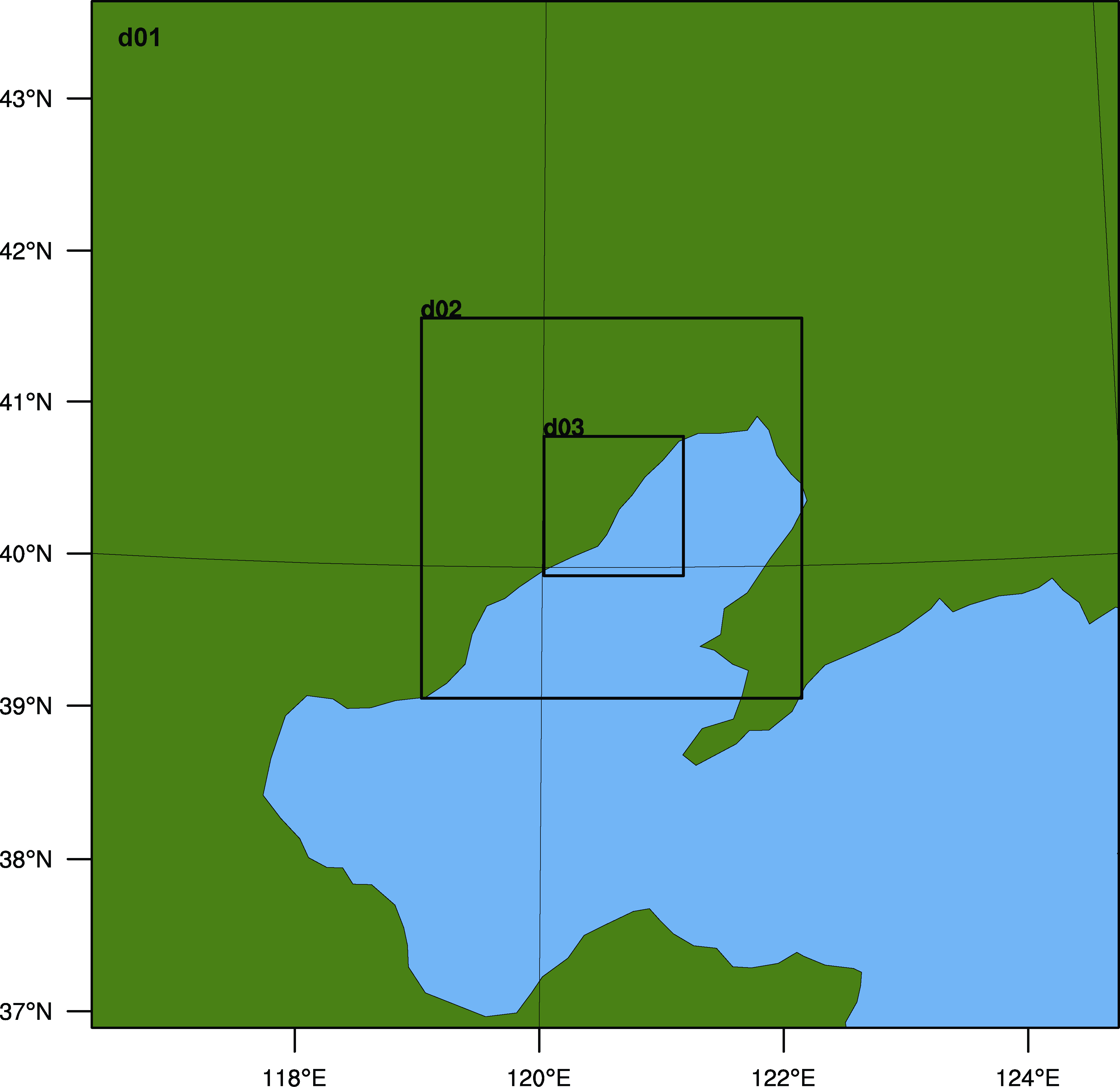	Figure 1 The Weather Research and Forecasting (WRF) model regional programs, the outside frame is domain one, on behalf of the northeast of China, the middle frame is domain two, situated at the area of the Bohai Bay, the inside frame is domain three, which represents the surrounding area of the wind farm. The wind farm is in the middle of this region.

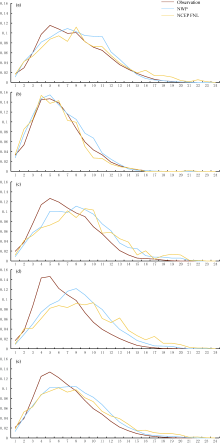
The wind speed probability density distributions obtained from the anemometer tower data, the WRF model simulation, and the FNL reanalysis data in spring, and especially in summer, were close to each other. Spring is the transition between winter and summer, so the weather systems move faster. The entire province frequently experiences windy weather because it is affected by alternating high and low pressure systems and changes of cold air. Usually, the wind speed in spring is higher than in the other seasons. It was clear that by downscaling the wind speed values found through the WRF model, the simulation values became closer to the observed values. Therefore, it can be concluded that the dynamical downscaling process was meaningful in terms of the wind speed values, which can be seen in Table 1. Downscaling is a method for obtaining high-resolution climate or weather change information from relatively coarse-resolution original material. Typically, the FNL data have a resolution of around 50-100 km, so the smaller-scale information needs to be estimated. The horizontal resolution in this study was 1 km, with a higher vertical resolution of 50 layers. Therefore, dynamical downscaling can use a limited-area, high-resolution model driven by boundary conditions to derive smaller-scale information. Obviously, the cut-out wind speed never appears.

Table 1

Table 1

Table 1 The relative frequency of wind speed (less than the value) by observation (Obs), numerical weather prediction (NWP), and National Centers for Environmental Prediction (NCEP) final (FNL) Operational Global Analysis data in four seasons and the whole year. Speed Spring Summer Autumn Winter Whole Year Obs WRF FNL Obs WRF FNL Obs WRF FNL Obs WRF FNL Obs WRF FNL 1 1.71% 1.12% 1.63% 3.29% 2.75% 3.40% 1.97% 0.89% 1.24% 1.65% 0.86% 0.97% 2.17% 0.13% 1.82% 2 2.95% 4.24% 4.22% 5.37% 7.46% 8.56% 3.77% 3.33% 4.12% 3.61% 2.88% 4.03% 3.95% 4.17% 5.24% 3 6.02% 5.98% 5.31% 10.28% 11.29% 10.46% 7.58% 5.74% 5.22% 8.64% 5.03% 4.17% 8.12% 6.54% 6.31% 4 9.71% 8.17% 6.95% 14.50% 14.75% 15.35% 11.38% 6.90% 6.73% 14.34% 7.39% 6.11% 12.45% 8.68% 8.81% 5 11.51% 9.07% 8.72% 14.68% 15.48% 13.72% 12.66% 10.05% 7.28% 14.63% 8.89% 8.19% 13.35% 10.19% 9.49% 6 10.80% 10.19% 9.40% 13.83% 13.45% 14.27% 11.92% 10.04% 8.10% 12.21% 9.74% 8.75% 12.20% 10.21% 10.14% 7 9.90% 1.09% 8.31% 11.56% 11.62% 10.33% 10.77% 9.83% 10.16% 10.88% 11.64% 8.33% 10.78% 10.38% 9.29% 8 10.04% 10.24% 11.17% 8.62% 10.47% 9.92% 9.72% 11.07% 8.79% 9.77% 12.17% 9.17% 9.53% 10.40% 9.77% 9 8.26% 9.48% 8.17% 5.92% 7.70% 5.03% 9.00% 10.43% 10.58% 7.29% 10.88% 8.89% 7.62% 9.14% 8.16% 10 7.10% 9.33% 7.22% 4.34% 6.72% 2.72% 6.91% 9.46% 10.30% 5.33% 9.25% 9.31% 5.93% 8.26% 7.37% 11 6.49% 9.29% 7.22% 3.33% 3.67% 2.58% 5.48% 7.51% 5.63% 3.93% 7.94% 6.11% 4.82% 6.77% 5.38% 12 5.01% 6.18% 5.45% 1.88% 2.45% 1.49% 3.74% 6.14% 5.77% 2.94% 5.73% 5.28% 3.39% 4.90% 4.49% 13 3.56% 4.65% 3.95% 1.15% 1.43% 0.95% 2.12% 3.65% 4.53% 2.08% 3.92% 6.25% 2.22% 3.26% 3.91% 14 2.63% 2.99% 2.86% 0.70% 0.51% 0.68% 1.24% 2.68% 3.85% 1.32% 2.84% 3.75% 1.47% 2.16% 2.78% 15 1.83% 1.57% 1.91% 0.33% 0.22% 0.41% 0.61% 2.52% 1.24% 0.68% 1.67% 2.64% 0.86% 1.44% 1.54% 16 1.20% 0.80% 2.45% 0.17% 0.13% 0 0.51% 1.07% 2.06% 0.39% 1.14% 1.81% 0.56% 0.76% 1.58% 17 0.62% 0.51% 1.36% 0.06% 0.07% 0 0.38% 0.80% 0.41% 0.18% 0.61% 2.50% 0.31% 0.48% 1.06% 18 0.32% 0.36% 1.36% 0 0.02% 0 0.21% 0.79% 1.10% 0.06% 0.55% 1.11% 0.15% 0.41% 0.89% 19 0.19% 0.14% 1.09% 0 0 0 0.06% 0.60% 1.37% 0.04% 0.48% 1.11% 0.07% 0.30% 0.89% 20 0.07% 0.10% 0.41% 0 0 0 ~ 0 0.60% 1.24% ~ 0 0.15% 0.83% 0.02% 0.21% 0.62% 21 0.04% 0.06% 0.14% 0 0 ~ 0 ~ 0 0.11% 0.14% 0 ~ 0 0.28% ~ 0 0.04% 0.17% 22 0.02% 0 0.54% 0 0 0 0 0 0.14% 0 0 0.14% ~ 0 0 0.21% 23 ~ 0 ~ 0 0.14% 0 0 0 0 0 0 0 0 0.14% ~ 0 ~ 0 0.06% 24 ~ 0 0 0 0 0 0 0 0 0 0 0 0 ~ 0 0 0 Although the results of the wind speed assessment in autumn and winter were not as close, it can be seen from Fig. 2 that they were still reasonably acceptable. The probability distribution curve ranged much wider than the observation result, with deviation to the right, and the overall evaluation of wind speed was higher. Finally, the mean whole-year wind speed probability density distribution was quite close, particularly when the downscaling WRF model was used to assess the basic wind speed probability density, but the deviation in autumn and winter still need to be analyzed.

Table 1 The relative frequency of wind speed (less than the value) by observation (Obs), numerical weather prediction (NWP), and National Centers for Environmental Prediction (NCEP) final (FNL) Operational Global Analysis data in four seasons and the whole year.

Figure 2

	Figure Option ViewDownloadNew Window
	Figure 2 Wind speed probability density distribution from observations, NWP, and NCEP FNL data in (a) spring, (b) summer, (c) autumn, (d) winter, and (e) the whole year. x-axis represents wind speed (m s-1).

If the power of the wind that flows at a speed ( v) through a blade sweep area can be expressed, then the calculation of the wind power density (WPD) based on the wind speed provided by field measurements can be developed using the following equations:

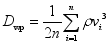, (1)

where ρ is the air density depending on altitude, air pressure, and temperature. n represents different periods of time required. It can also be seen from Eq. (1) that WPD increases with the cube of the wind speed ( Islam et al., 2011). The effective WPD can be calculated as:

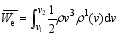, (2)

where v₁ is the cut-in speed and v₂ is the cut-out speed. ρ¹( v) represents wind speed probability density.

The wind resource assessment was calculated using statistical techniques, which allowed an estimate of the amount of electrical energy produced by a specific wind turbine using time series data. This first calculation provided a fundamental element to determine the economical feasibility of the site as a producer of electricity using the wind resource ( Rodrigues-Hernandez et al., 2013). Table 2 shows that in spring the wind speed is higher than in the other three seasons, and that the mean wind speed at a height of 70 m was over 7 m s^?1. The minimum wind speed was less than 6 m s^?1. The effective wind speed needs to be more than 3 m s^?1 and less than 25 m s^?1. The maximum hours of winds between these speeds appeared in spring and summer, but there was a lack of observation data and some errors, which were slightly less in winter. Overall, the annual effective wind hours for that region was more than 7200 hours. The lowest percentage of effective wind speed was 81.1%, while the effective wind speed in the remaining three seasons exceeded 85%, with a high availability. The WPD is required for the estima- tion of power potential from wind turbines ( Morrissey and Cook, 2009). In spring, the average wind power density at a height of 70 m was greater than 400 W m^-2, and the effective wind power density was more than 450 W m^-2, but in summer the mean wind power density was lower than 200 W m^-2. In general, the annual average WPD at a height of 70 m was more than 300 W m^-2. The effective WPD and the hours of effective wind speed were both high, as this region is in a wind-energy-rich area.

Table 2

Table 2

Table 2 Key parameters from the anemometer tower and mesoscale NWP at 70 m in each season. In each case, data from the anemometer tower are shown on the left, and the numerical simulation on the right (separated by the solidus). In wind direction column, east (E), west (W), south (S), north (N). Para- meters Average wind speed at 70 m (m s-1) Wind direction occurs more at 70 m Average hours of effective wind speed (h) Percentage of effective wind speed Average WPD (W m-2) Average effective WPD (W m-2) Spring 7.11/7.47 SSW, SW, N, NNE /SSW, SW, S, NNE 1889/1890 85.60%/89.23% 411.64/442.52 460.1/495.13 Summer 5.43/5.60 SSW, SW, S, N /SSW, S, SW, SSE 1775/1670 81.10%/80.5% 183.87/197.75 225.43/244.14 Autumn 6.40/7.74 SSW, SW, N, NNE /N, SW, SSW, NNE 1888/1965 86.70%/90.44% 297.15/511.06 341.68/564.38 Winter 6.03/7.65 NNE, NE, SW, SSW /N, NNW, NNE, WSW 1664/1945 86.10%/91.55% 263.86/481.05 305.29/524.83

Table 2 Key parameters from the anemometer tower and mesoscale NWP at 70 m in each season. In each case, data from the anemometer tower are shown on the left, and the numerical simulation on the right (separated by the solidus). In wind direction column, east (E), west (W), south (S), north (N).

In summary, the mean wind speed from the WRF model was higher than from the observation tower; the wind speed in autumn was highest, then in winter, and it was lowest in summer. The mean wind speed in autumn and winter was higher than in spring, which was significantly different from the tower measurements. There was a large deviation between the two methods in autumn and winter, especially as the effective hours exceeded 90% from the NWP model, and could be as high as 91.55% in winter. For the NWP model, the average wind power density was higher than 510 W m^-2 in autumn, which exceeded the observation data; the effective wind power density was higher by 65%. The index was significantly higher than the observation assessment in autumn and winter.

Regardless of the wind speed, wind direction, or wind power density, there was an obvious difference between the simulations and observations in autumn and winter, so it is intriguing why the results simulated by the mesoscale NWP model overestimated the wind energy of that region in those two seasons. Though utilizing NWP models to assess wind resources has become a mainstream method, its validity still needs to be questioned.

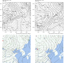
Some parameters were significantly different between the two methods, so we further analyzed why the values from the numerical simulation were higher than the observations from the anemometer tower. Wind power depends on the weather and the climate, as well as the wind farm itself ( Zhou et al., 2013), so there is a need to analyze the typical weather patterns to explain the problem. In autumn and winter, cold northerly winds behind cold fronts are a major factor in this province, so we chose a typical weather process to analyze the situation. First, using the WRF model, a cold windy synoptic-scale weather process was simulated; we used a Mongolian cold high pressure coming down from the northwest. The strength of the high pressure center was more than 1030 hPa, and there was a low pressure circulation in the south to the northeast. When the two circulations were superimposed, the isobars became denser, which enhanced the pressure gradient force and increased the wind speed. It can be seen from Fig. 3 that the wind farm was located in a dense isobar area from 0000 UTC to 1800 21 UTC September 2010, with a higher wind speed. This verifies that the area was subjected to cold windy weather through the observations from the anemometer tower. There were certain differences between the observation results and the simulation synoptic-scale weather, but the difference in the change of the low pressure circulation existed. As can be seen from the simulation results, the southern low pressure moved eastward, and its central pressure increased from 1008 hPa to 1012 hPa, with a certain level strengthened. However, the observations showed that the pressure change from 1008 hPa to 1010 hPa quickly dissipated. The strengthening process was almost negligible, which made the pressure gradient predicted by the mesoscale NWP model higher, and this obviously made the wind speed higher than the measured wind speed.

Figure 3

	Figure Option ViewDownloadNew Window
	Figure 3 The sea level pressure (SLP) and ground 10-m wind from (a, b) numerical simulation and (c, d) meteorological stations from (a, c) 0000 UTC 21 September 2010 to (b, d) 1800 UTC 21 September 2010.

In this study, WRF model simulations and anemometer tower observations were used to assess the Liaoning coastal wind farm. This provided an objective verification of the two methods against which future model improvements may be measured. Overall, the WRF model using dynamical downscaling can effectively assess the region’s wind power, but the values of the parameters from the mesoscale NWP model were higher than the measurements from the wind tower. Since there were significant differences between the two methods in autumn and winter, further research is necessary. Through analyzing some typical synoptic-scale changes, it was found that the high and low pressure simulated by the numerical model was relatively stronger and slightly slower, leading to the area being affected by a large pressure gradient lasting for a longer time. This meant that the forecasted strength of the large-scale circulation was higher, so the wind speed prediction was higher. This wind farm is located in the southwest of Liaoning Province, which is usually influenced by cold windy weather in autumn and winter. Due to the model’s overestimation of the intensity and duration of the windy weather, the wind speed given by the mesoscale NWP model in these two seasons is too high.

Finally, the initial data and the prediction process of the WRF model can lead to a large deviation in the wind power assessment. The mesoscale NWP-WRF model can be used to assess the wind energy resources through the dynamical downscaling process, but it should not be overly relied upon. Observational data, such as the anemometer tower measurements, should be used together with simulated analysis and evaluation.