

A New Method for Aerosol Retrieval Based on Lidar Observations in Beijing
[PAN Yu-Bing1, 2 , LÜ Da-Ren1 , PAN Weilin1  ]
]
]
|
|


Lidar has been used extensively in the area of atmospheric aerosol measurement. Two unknowns at the reference altitude, the lidar ratio and the backscatter coefficient, need to be resolved from the lidar equation. In the actual application, these two values are difficult to obtain, particularly the backscatter coefficient. To better characterize the optical properties of aerosols, optical thickness, and attenuated backscatter obtained by other instruments are usually used as the input for joint inversion. However, this method is limited by location and time. In this study, the authors propose a new method for aerosol retrieval by using Mie scattering lidar data to solve this problem. The authors take the horizontal aerosol extinction coefficient as the constraint to begin the iteration until a self-consistent aerosol vertical profile was obtained. By comparing their results with Aerosol Robotic Network (AERONET) data, the authours determine that the aerosol extinction coefficient obtained by combining horizontal and vertical lidar observations is more precise than that obtained by using the traditional Fernald method. This new method has been adopted for retrieving the extinction coefficient of aerosols during the observation days.
Aerosols play an important role in atmospheric radiation and climate change. They can affect the radiation balance of the earth-atmosphere system by absorbing and scattering solar radiation, which is known as the direct radiation effect. Aerosols can also act as cloud condensation nuclei during the cloud generation process, thereby changing the physical characteristics and radiation properties of the cloud, which is known as the indirect radiation effect ( Twomey, 1977; Lohmann and Feichter, 1997). By using advanced atmospheric remote sensing technology to conduct in-depth study of the spatial and temporal distribution of aerosol concentration and its physical and chemical properties, aerosol climate effects research can be quantified with continuous improvement of the climate models.
As an active remote sensing tool, lidar has been used extensively in the field of atmospheric and environmental research, primarily in detecting the optical properties of aerosols and cirrus clouds in the troposphere.
Welton et al. (2000) used micropulse lidar to obtain aerosol vertical distribution and physical properties in the Aerosol Characterization Experiment 2 (ACE-2) and compared their results with those obtained by other ground-based instruments and satellite data. The Atmospheric Radiation Measurement (ARM) program supported by the U.S. Department of Energy (DOE) obtained atmospheric observational data by using various ground- based instruments such as lidar to better understand the clouds and aerosols processes in climate system models, as well as their interactions ( Campbell et al., 2002).
In their study of solving lidar equations, Dulac and Chazette (2003) calculated the column-averaged lidar ratio (LR) by comparing the aerosol optical depth (AOD) retrieved from the Meteosat satellite with that obtained from lidar. Their results showed that the average LR is quite accurate. Welton et al. (2002) presented an iterative method based on the aerosol optical thickness from independent observations as a limiting factor. This method can not only obtain the aerosol extinction coefficient and AOD but also can calculate LR. Lu et al. (2011) purposed a retrieval method by combining ground-based and space-borne lidar observations. This technique can obtain the aerosol extinction coefficients and aerosol extinction-to-backscatter ratio in more than one aerosol layer. They compared their results with data from Cloud Aerosol Lidar and Infrared Pathfinder Satellite Observations (CALIPSO) and Napoli-Earlinet lidar data and reported a good agreement.
However, previous studies often rely on other instrument data for solving lidar equations. In the present study, we propose a new method by using a single lidar to obtain the aerosol vertical profiles.
In recent years, many universities and research institutions have successfully developed lidar systems. The lidar used in the present study is a Mie scattering lidar system manufactured by Xi'an University of Technology ( Yan et al., 2013) installed at the top of Building No. 40, Institute of Atmospheric Physics, Chinese Academy of Sciences (39.97°N, 116.38°E).
This lidar system contains a diode pumped Nd: YAG laser with a pulse output at a wavelength of 532 nm. The pulse duration is 12 ns with a pulse repetition frequency (PRF) of 1 kHz, and the pulse energy is approximately 50 μJ. This lidar runs on the analog detection mode, which is more suitable than the photon counting mode for monitoring high-concentration aerosols in urban areas. The receiving telescope, with a 254 mm diameter and a 2500 mm focal length, has a ground-penetrating radar system (GPRS) scanning function with azimuth angles from 0° to 360° and zenith angles from 0° to 90°. The specifications of this micro-pulsed Mie scattering lidar are shown in Table 1.
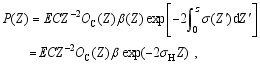
Aerosol optical properties can be determined by lidar return signals. Under the assumption of evenly mixed air, we can use Collis slope method to solve the laser radar equation ( Collis and Russell, 1976). However, if the air along the laser propagation path changes significantly, Klett method ( Klett, 1985) and the Fernald method ( Fernald, 1984) must be used. In the present study, we use mainly the Fernald method for the inversion of the lidar equation, which divides the lidar signals into those from the air molecules and those from aerosols. The lidar equation is written as follows:

In the above equation, P(Z) is the energy received by the lidar at the height of Z, E represents the lidar emission energy, C is the lidar instrument parameter, 

We can use the backward integration method to solve the equation:
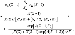
where 


| Table 1 Specifications of micro-pulsed Mie scattering lidar. |
| Table 2 Aerosol lidar ratio categorized from the Cloud-Aerosol Lidar with Orthogonal Polarization (CALIOP) aerosol model. |
For an additional unknown 
We conducted Mie Lidar observations in both horizontal and vertical directions. The fundamental criterion of choosing horizontal observation time is to include the time period during which the atmospheric condition is stable, with weak surface wind and clear air ( Welton, 2002).
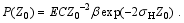
Assuming the atmosphere is evenly mixed horizontally, the atmospheric extinction coefficient and the volume backscattering coefficient are constant. The lidar equation in the horizontal direction can be written as
where 

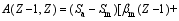
If the laser beam fully entering the receiving telescope's field of view starts from altitude 

Form these two equations, we can get the expression of geometric form factor as

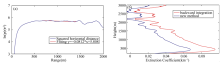
Figure 1a shows the geometric form factor obtained in the experiment. This factor increases as a function of distance until 600 m, where the receiver's field of view is completely overlapped with the laser beam. The geometric form factor does not change with time, which shows the consistency and stability of the lidar performance.
Although the horizontal atmosphere cannot be completely mixed evenly, we can obtain the atmospheric extinction coefficient in a short distance by using the adaptive least squares method. As shown in Fig. 1a, the receiver's field of view does not completely overlap with the laser until 600 m; therefore, least squares fitting is performed on the horizontal data from 600 m to 3000 m. To find a more qualified curve, the fitting is started from 600 m with integration steps of 100 m, and the least squares fitting method is applied to determine the minimum variance, which is the best fitting range.
By using this method, we can obtain the horizontal atmospheric extinction coefficient, as shown in Fig. 1b, with 
We selected the vertical observation data within 30 min from the horizontal observation. The atmospheric condition is assumed to be stable during this time period.
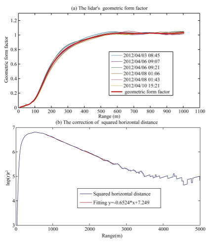 | Figure 1 Plots of (a) geometric form factor and (b) ln p(r)r2 as functions of range in the horizontal observation ( p(r) is the energy received by the lidar at the height of r). |
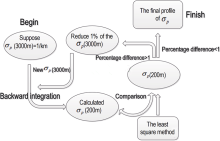
Because the lidar observation capability is limited to the lower troposphere in daytime, we selected 3000 m as the starting point of the inversion. The aerosol extinction coefficient obtained from horizontal observation is taken as the aerosol extinction coefficient at an altitude of 200 m. Figure 2 shows our calculation procedure. We suppose the aerosol extinction coefficient at 3000 m altitude is 1 km-1, then we use the backward integration method to retrieve the data. After calculating the aerosol extinction coefficient at the 200 m altitude, we compared the results with the aerosol extinction coefficient from horizontal observation. If the difference is less than 1%, we take the supposed extinction coefficient as the actual value at 3000 m. Otherwise, we reduce 1% of the extinction coefficient and conduct this iteration until the difference is less than 1%.
 | Figure 2 Flow chart of iterative computation of extinction coefficient. |
We selected data obtained on 7 February, 8 February, and 10 February 2013, which were clear days. Horizontal lidar measurements were conducted during those days during the daytime according to the experiment requirement.
Equation (5) was used to compute the horizontal aerosol extinction coefficient at 15:54 local time (UTC+8) on 7 February 2013, because the atmosphere was very clean during this period. Figure 3a shows the correction of squared horizontal distance. By using the square method, the atmospheric extinction coefficient at the horizontal direction was determined to be 0.0405 km-1; we then obtained the aerosol extinction coefficient as 0.0276 km-1.
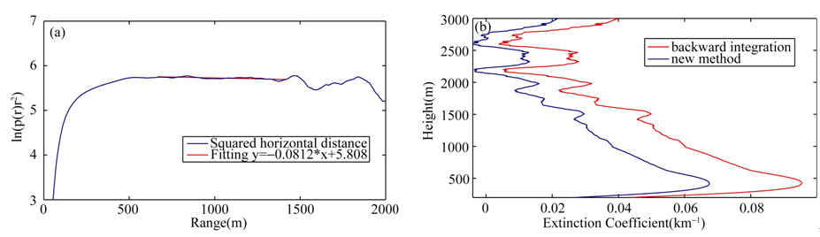 | Figure 3 Plots of (a) ln p(r)r2 as a function of range in horizontal observation recorded on 15:54 7 February 2013 local time. (b) Plot of aerosol retrieval by using backward integration and the new method for data recorded at 16:08 on the same day. |
In addition, we compared the unconstrained backward integration method with this new method. Due to the lack of long-term continuous aerosol observations in Beijing, the background atmospheric aerosol extinction coefficient in the Hefei area was taken as the boundary value ( Zhou et al., 1998) in the backward integration calculation. As shown in Fig. 3b, the two profiles have similar shapes, with the aerosol extinction coefficient larger near the surface and decreasing with altitude. Moreover, the result obtained from backward integration method (plotted in red) is noticeably larger than that from our new method (plotted in blue). On the basis of the new method, the aerosol extinction coefficient at 3000 m was determined to be 0.0206 km-1, and the aerosol extinction coefficient at 200 m was 0.0275 km-1 According to the empirical values, the aerosol extinction coefficient at 3000 m was 0.0376 km-1, and aerosol extinction coefficient at 200 m was 0.0429 km-1. The difference was larger at higher altitudes.
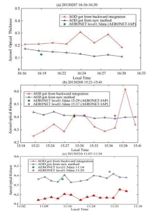
As shown in Fig. 4, we compared these two results with AERONET data (http://aeronet.gsfc.nasa.gov/). The AERONET Beijing site's Cimel heliograph is stationed at the top of Building No. 40, Institute of Atmospheric Physics, Chinese Academy of Sciences (AERONET-IAP), at the same location as that of the Mie lidar. The AERONET Level 1.5 product data, which have been cloud cleared, were selected for comparison. The AOD above 3 km was replaced by the background atmospheric aerosol extinction coefficient in the Hefei area ( Zhou et al., 1998). Because few aerosols are present above 3 km during a clear day, their difference was negligible.
AOD was calculated to be 0.1256 on 16:19 7 February 2013 local time. As shown in Fig. 4a, the AOD obtained from the new method is closer to AERONET data (0.125592) than that from backward integration. The minimum difference was 0.0026 at 16:28 local time, and the maximum difference was 0.0463 at 16:16 local time. All differences were less than 0.05.
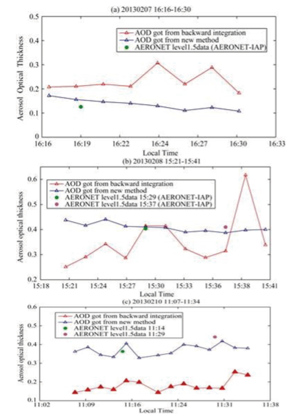 | Figure 4 Comparison of aerosol optical depth (AOD) obtained from backward integration and the new method with AERONET level 1.5 data recorded on (a) 7 February 2013, (b) 8 February 2013, and (c) 10 February 2013. |
As shown in Figs. 4b and 4c, the same computation was applied to the data of 8 February 2013 and 10 February 2013. The results again show that the AOD obtained from the new method is closer to AERONET data than that from backward integration.
The mean aerosol extinction coefficient was obtained during the observation days by using this method (Fig. 5). Aerosols are mainly gathered 2 km above the surface. We determined that although the extinction coefficient near the ground surface is small, it increases with an increase in height and reaches its maximum near the top of the boundary layer. This phenomenon is attributed to many reasons, such as the inversion layer, misty rain effect, and the relative humidity. Above 2 km, the curve presented attenuation distribution. The aerosol extinction coefficient at 3 km was 0.0334 km-1.
Errors may arise from the estimation of the horizontal extinction coefficient and lidar ratio ( Fernald, 1984). To obtain a more accurate horizontal extinction coefficient, we fit the assumed evenly mixed atmosphere by using the least squares method. The uncertainty of the lidar ratio is no more than 30% ( Omar et al., 2009). In addition, the backscatter coefficient is insensitive to the lidar ratio Chen et al., 2011). Considering that the entire extinction coefficient on clear days is small, this effect has little impact on the inversion.
Two unknown quantities are to be resolved from lidar equations: lidar ratio and backscatter coefficient at a given height. Although the tropopause is generally chosen as the altitude for calibration, in actual application, lidar detectability is limited to the lower troposphere in daytime. Joint inversion with optical thickness and attenuated backscatter simultaneously measured by other instruments could be used; however, not all lidar sites have such extra data available. In this study, we purposed a new method for solving this problem.
We conducted horizontal observation under stable weather conditions and calculate the upper atmospheric extinction coefficient by using the adaptive least squares method. We then used the results as the constraint to begin the iteration until we obtained a self-consistent aerosol vertical profile. Finally, we compared the results with AERONET data and the results of traditional backward integration, and we demonstrated that our results are closer to the AERONET data.
Although, this new method is suitable for use under relatively stable weather conditions, it may not perform well on windy or dusty days. Further study is required to determine methods for precise calculation of the extinction coefficient under different weather conditions. Moreover, it should be noted that we have conducted only a few experiments and calculations. To improve this new method, additional experiments should be designed in future studies.
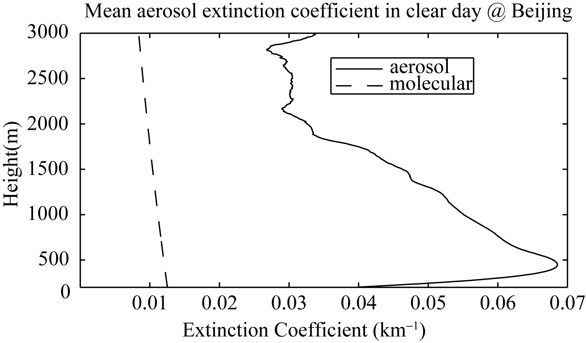 | Figure 5 Mean aerosol extinction coefficient obtained during the observation days in Beijing. |
| 1 |
|
| 2 |
|
| 3 |
|
| 4 |
|
| 5 |
|
| 6 |
|
| 7 |
|
| 8 |
|
| 9 |
|
| 10 |
|
| 11 |
|
| 12 |
|
| 13 |
|
| 14 |
|
| 15 |
|
| 16 |
|