

 N, 126°10
Initial Results of Lidar Measured Middle Atmosphere Temperatures over Tibetan Plateau
[QIAO Shuai1, 2 , PAN Weilin1  , ZHU Ke-Yun
2 , ZOU Rong-Shi1 , TAN Jing1, 2 ]
, ZHU Ke-Yun|
|


During August 2013, a mobile Rayleigh lidar was deployed in Lhasa, Tibet (29.6°N, 91.0°E) for making measurements of middle atmosphere densities and temperatures from 30 to 90 km. In this paper, the authors present the initial results from this scientific campaign, Middle Atmosphere Remote Mobile Observatory in Tibet (MARMOT), and compared the results to the MSIS-00 (Mass Spectrometer and Incoherent Scatter) model. This work will advance our understanding of middle atmosphere dynamic processes, especially over the Tibetan Plateau area.
Temperature is a key factor for understanding the chemical, dynamic, and radiative processes in the atmosphere. The thermal structure in the middle atmosphere has a close connection with atmospheric ozone and related photochemical reactions. However, atmospheric temperature is affected by waves (gravity waves, tides, and planetary waves) and atmospheric circulation Lü and Chen, 2003; Wang, 2011). Observations and modeling indicate gradual cooling in the middle atmosphere ( Ramaswamy et al., 2001), and the formation of mid-latitude noctilucent clouds may be a harbinger of global climate change ( Herron et al., 2007). Therefore, temperature profiling is of great importance for studying middle atmosphere temperature variations and for validating the current atmospheric models ( Pan and Gardner, 2002).
The middle atmosphere between 30 and 90 km is higher than the detectable range for aircraft and sounding balloons. Rocket can probe one vertical profile at a certain point in time, and the cost is relatively high ( Keckhut et al., 1995). But Rayleigh lidar, with its high spatial and temporal resolution ( Chanin, 1984; Gobbi et al., 1995; Yan, 2001), is an effective means for measuring vertical temperature profiles in the middle atmosphere ( Shibata et al., 1986; Gardner, 1989, 2001; Hauchecorne and Chanin, 1991; Hauchecorne et al., 1992).
The Middle Atmosphere Remote Mobile Observatory in Tibet (MARMOT) lidar was recently developed by the Institute of Atmospheric Physics (IAP), Chinese Academy of Sciences (CAS). In this paper, we will describe the MARMOT lidar system and our lidar data retrieval method, and show some preliminary results of middle atmosphere temperature measurements over Lhasa, Tibet.
The MARMOT lidar consisted of three parts: laser transmitter unit, optical receiver unit, and signal acquisition & control unit. A block diagram of the MARMOT lidar system is shown in Fig. 1.
 | Figure 1 Block diagram of the MARMOT lidar system. |
The main part of the laser transmitter was a Nd:YAG laser working at wavelengths of both 532 nm and 1064 nm. The optical receivers were a prime focus telescope of Ф1000 mm diameter and a Newtonian telescope of Ф200 mm diameter. Lidar backscattered signals of 532 nm and 1064 nm were collected by the prime focus telescope and then detected by one Photomultiplier Tube (PMT) and one Avalanche Photodiode (APD), respectively. The Newtonian telescope and another PMT received lidar signals of 532 nm. Signals from these optical detectors were then collected by transient recorders and stored as binary files in the computer.
In MARMOT lidar system, we used dual telescope configuration to collect the 532 nm signals. Signals received by the large-aperture prime focus telescope covered the 50-90 km altitude range. An optical chopper in the receiver blocked lidar signals below 50 km in order to avoid PMT saturation caused by strong lidar return signals from low altitudes. For signals below 50 km, we used a Newtonian telescope with smaller aperture. During this experiment, the high-altitude 532 nm signal could reach 50-90 km, and the low-altitude 532 nm signal could reach 30-60 km. Thus, we were able to obtain a 532 nm Rayleigh signal profile for altitudes between 30 and 90 km. Results from the 1064 nm signal are not discussed in this paper. The system specifications for the MARMOT lidar are shown in Table 1.
| Table 1 Specifications of the MARMOT lidar system. |
The main principle of Rayleigh temperature derivation is as follows. Considering that the aerosol content is extremely low above 30 km, the lidar backscattered signal mainly comes from Rayleigh scattering by gaseous molecules. By calculating the atmospheric backscattered signals, we can get the relative density profile in the atmosphere. If we assume the atmospheric temperature at a higher altitude (~ 90 km, in our case) can be taken from the Mass Spectrometer and Incoherent Scatter (MSIS-00) model, then by combining the ideal gas law and the hydrostatic equation, atmospheric temperature profiles can be derived from relative density profiles ( Hauchecorne and Chanin, 1980; Liu et al., 2006).
In August 2013, the MARMOT lidar was operated in Lhasa, Tibet (29.6°N, 91.0°E), for 23 days, obtaining approximately 135 h of valid data. In this paper, we used 1-h lidar data between 22:20 and 23:30 local time (LT) on 22 August 2013 to derive and analyze the middle atmosphere density and temperature over Lhasa. These 1-h lidar data were chosen for their relatively high signal to noise ratio (SNR) and relatively stable background noise.
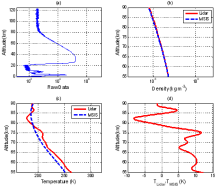
Figure 2a shows the high-altitude 532 nm signal, representing the raw photon counts from 50 to 90 km. The derived density and temperature are plotted in Figs. 2b and 2c, respectively. The differences between temperatures derived from lidar ( Tlidar) and temperatures from the MSIS-00 model ( TMSIS) are shown in Fig. 2d. We can see that the derived temperature and MSIS-00 temperature agreed well for altitudes of 55-80 km, while the derived temperature was slightly warmer than the MSIS-00 model above 80 km. The derived temperature was 1-12 K warmer than the model from 55 to 78 km and 85 to 88 km, but was 1-8 K colder than the model from 79 to 85 km.
 | Figure 2 Observation results from the high-altitude 532 nm channel on 22 August 2013: (a) raw photon counts from lidar measurements, (b) density profiles, (c) temperature profiles, and (d) the difference between lidar measured temperature and MSIS-00 temperature. In (b) and (c), red solid line for lidar measurements, blue dashed line for MSIS-00 model. |
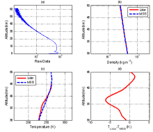
Figure 3a shows the low-altitude 532 nm signal, representing raw photon counts from 30 to 60 km. The derived density and temperature are plotted in Figs. 3b and 3c, respectively. The differences between Tlidar and TMSIS are shown in Fig. 3d. We can see that the derived temperature and MSIS-00 temperature agreed well from 30 to 45 km. The derived temperature was 1-7 K colder than the model from 30 to 40 km.
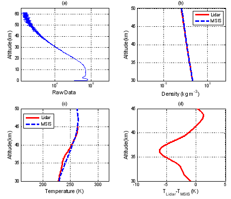 | Figure 3 Observation results from the low-altitude 532 nm channel on 22 August 2013: (a) raw photon counts from lidar measurements, (b) density profiles, (c) temperature profiles, and (d) the difference between lidar measured temperature and MSIS-00 temperature. In (b) and (c), red solid line for lidar measurements, blue dashed line for MSIS-00 model. |
We combined the smoothed high-altitude 532 nm (from 50 to 90 km) and low-altitude 532 nm signals (from 30 to 60 km) together using normalization method, that is, by normalizing the high-altitude 532 nm signals and the low-altitude 532 nm signals by their corresponding signal levels at a certain altitude (~ 51 km, in our case), and then "stitching" them together to obtain a continuous altitude coverage of 532 nm lidar signals from 30 to 90 km. Then, the relative photon counts for this altitude range are plotted in Fig. 4a. Figure 4b shows the derived density pro file. Figure 4c shows the derived temperature profile for this 1 h observation period, as well as the monthly mean lidar temperature profile obtained during 8-24 August 2013 in Lhasa. The differences between Tlidar and TMSIS are plotted in Fig. 4d. Between 55 and 80 km, the derived temperature agreed well with the model. Tlidar was 1-18 K warmer than TMSIS between 42 km and 79 km, but 1-7 K colder from 30 to 42 km and 79 to 85 km.
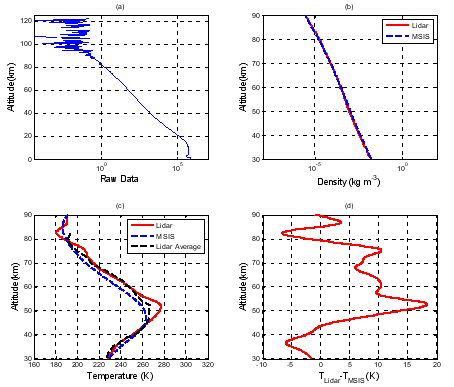 | Figure 4 The results combining the high-altitude 532 nm and the low-altitude 532 nm channels on 22 August 2013: (a) raw photon counts from lidar measurements, (b) density profiles, (c) temperature profiles, and (d) the difference between lidar measured temperature and MSIS-00 temperature. In (b) and (c), red solid line for lidar measurements, blue dashed line for MSIS-00 model. |
Our MARMOT lidar has made successful measurements of middle atmosphere density and temperature profiles in Lhasa, Tibet. The derived lidar temperatures from 30 km to 90 km ranged from 7 K colder to 18 K warmer than the MSIS-00 model. This discrepancy could be caused by atmospheric waves, and/or the inaccuracy of the MSIS-00 model. Our preliminary results have suggested some limitations of the MSIS-00 model, since the model was developed under the circumstances that not much middle atmosphere observational data was available over the Tibetan Plateau. Therefore, lidar measurements could provide an effective tool for improving current atmospheric modeling. Furthermore, lidar observational data could become a unique dataset for better understanding the middle atmosphere thermal structure, the waves, and the processes of momentum and energy exchange within layers. We plan to upgrade our lidar system by improving data quality and by extending altitude coverage.
| 1 |
|
| 2 |
|
| 3 |
|
| 4 |
|
| 5 |
|
| 6 |
|
| 7 |
|
| 8 |
|
| 9 |
|
| 10 |
|
| 11 |
|
| 12 |
|
| 13 |
|
| 14 |
|
| 15 |
|
| 16 |
|