

Aerosol Type Identification Using PARASOL Multichannel Polarized Data
[FAN Xue-Hua , CHEN Hong-Bin]
, CHEN Hong-Bin]
|
|


PARASOL (Polarization & Anisotropy of Reflectances for Atmospheric Sciences coupled with Observations from a Lidar) multi-channel and multi-directional polarized data for different aerosol types were compared. The PARASOL polarized radiance data at 490 nm, 670 nm, and 865 nm increased with aerosol optical thickness (AOT) for fine-mode aerosols; however, the polarized radiances at 490 nm and 670 nm decreased as AOT increased for coarse dust aerosols. Thus, the variation of the polarized radiance with AOT can be used to identify fine or coarse particle-dominated aerosols. Polarized radiances at three wavelengths for fine- and coarse-mode aerosols were analyzed and fitted by linear regression. The slope of the line for 670 nm and 490 nm wavelength pairs is less than 0.35 for dust aerosols. However, the value for fine-mode aerosols is greater than 0.60. The Support Vector Machine method (SVM) based on 12 vector features was used to discriminate clear sky, coarse dust aerosols, fine-mode aerosols, and cloud. Two cases were given and validated by AErosol RObotic NETwork (AERONET) measurements, MODIS (Moderate Resolution Imaging Spectroradiometer) FMF (Fine Mode Fraction at 550 nm) images, PARASOL RGB (Red Green Blue) images, and CALIOP (Cloud-Aerosol Lidar with Orthogonal Polarization) VFM (Vertical Feature Mask) data.
Aerosols affect the earth's climate by scattering and absorbing radiation and by altering cloud microphysics. Aerosols have different scattering and absorption properties depending on their origin, and it is important to identify them in order to better quantify their radiative impact ( Niang et al., 2006). Partitioning of mineral dust, pollution, smoke, and mixtures using remote sensing techniques can help improve accuracy of data retrieved from satellites and assessments of aerosols' radiative impact on climate ( Giles et al., 2012). Since the type of aerosol can affect measurements of reflectance at the top of the atmosphere (TOA), aerosol type classification from satellite remote sensing is challenging. There have been a limited number of studies of classification of aerosols from satellite data compared with studies of aerosol amounts and optical properties. Higurashi and Nakajima (2002) developed a four-channel algorithm to classify aerosols into four major aerosol types-soil dust, carbonaceous, sulfate, and sea salt aerosols-using the data of space- borne multi-spectral ocean-color sensors (SeaWiFS) over the ocean. Jeong and Li (2005) developed an aerosol-classifying algorithm by utilizing two instruments: the Total Ozone Mapping Spectrometer (TOMS) and the Advanced Very High Resolution Radiometer (AVHRR). Aerosol size (the Angstrom exponent) from AVHRR and aerosol absorption (aerosol index) from TOMS were combined to classify aerosol types as either biomass burning particles, pollution, dust, sea salt, or mixtures of these types. Hsu et al. (2004) developed the Deep Blue algorithm, in which three channels were used to distinguish smoke and dust over bright-reflecting source regions. Niang et al. (2006) developed a method to determine aerosol type and thereby retrieve optical thickness from TOA reflectance measurements by SeaWiFs based on a neural network classification methodology. There have been other attempts to infer aerosol types, for example, from data from the Multi-angle Imaging Spectro-Radiometer (MISR) ( Martonchik et al., 1998), and POLarization and Directionality of the Earth's Reflectance (POLDER) ( Bellouin et al., 2003).
In this study, we investigated the possibility of inferring fine- and coarse-mode aerosol types from anthropogenic and natural sources, respectively, using TOA radiance and polarized radiance spectra from the Polarization & Anisotropy of Reflectances for Atmospheric Sciences coupled with Observations from a Lidar (PARASOL) satellite.
The PARASOL satellite is a part of the so-called"A-train"eries and carries the POLDER-3 instrument consisting of wide-field-of-view telecentric optics, a rotating wheel with spectral and polarizing filters, and a 274×242 two-dimensional Charge Coupled Device (CCD) detector array ( Deschamps et al., 1994). The polarization measurements were performed at three wavelengths (490, 670, and 865 nm). Three elements of the Stokes parameter ( I, Q, and U) were obtained. The directional measurements spanned up to 51° in the along-track direction and up to 43° in the cross-track direction. The ground pixel size is about 5×6 km2 at the nadir. Multiple angle viewings were obtained by overlapping successive images of the same spectral band. Thus, in a single satellite pass, any target within the instrument's purview could be observed quasi-simultaneously from up to 16 viewing angles.
The POLDER/PARASOL level 1 data used in this study were radiometrically calibrated and geometrically corrected. The normalized polarized radiance, Lp, is defined by the second and third Stokes parameters ( Q and U) as follows:
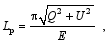
where Eis the spectral solar intensity at the TOA. The first Stokes parameter, I, can determine total radiance, L:

The satellite viewing geometry and some auxiliary data were also included in the level 1 data. The scattering angle, 

where 


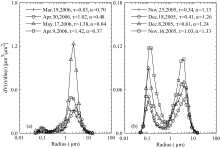
Direct and diffuse spectral radiances were measured by the ground-based CIMEL CE318 sunphotometer in Beijing (39.98°N, 116.38°E), an AERONET radiometer, and the PHOtométrie pour le Traitement Opérationnel de Normalisation Satellitaire (PHOTONS) station. The measurements were used to derive aerosol physical and optical properties, such as Aerosol Optical Thickness (AOT), size distribution, single scattering albedo, etc., based on the algorithm of Dubovik and King (2000). According to the AERONET AOT and Angstrom Exponent (AE) data in Beijing, two aerosol types were selected. One type was fine-mode aerosol with AE (440-870 nm) > 1.10; the other was dust aerosol with AE < 0.80. The AOT at 490, 670, and 870 nm and AE (440-870 nm) associated with the two aerosol types are shown in Table 1.
The volume size distribution of AERONET/PHOTONS data for coarse-mode dust cases and fine-mode pollution cases are shown in Figs. 1a and 1b, respectively. It can be seen in Fig. 1a that coarse particles (particle radius > 1 μm) are dominant for the dust cases, and fine particles (particle radius < 0.6 μm) are dominant for the fine mode pollution (Fig. 1b).
| Table 1 The Aerosol Robotic NETwork (AERONET) Aerosol Optical Thickness (AOT) at 490, 670, and 870 nm and Angstrom Exponent (AE) (440-870 nm) for coarse-mode dust cases (AE < 0.80) and fine-mode pollution cases (AE > 1.10). |
 | Figure 1 AERONET aerosol volume size distribution for Beijing (a) coarse dust days and (b) fine-mode pollution days; τ is AOT at 490 nm and α is AE at 440 and 870 nm. |
Support vector machines (SVMs) are a group of supervised learning models that can be applied to classification or regression and have exhibited excellent performance in many classification applications ( Vapnik, 1999; Suykens, 2001). The basic SVM takes a set of input data and predicts, for each given input, which of two possible classes forms the output, making it a non-probabilistic binary linear classifier. Given a set of training samples, each marked as belonging to one of two categories, an SVM training algorithm builds a model that assigns new samples into one category or the other. Multiclass SVM aims to assign labels to instances by using support vector machines, where the labels are drawn from a finite set of several elements.
The typical approach is to reduce the single multiclass problem into multiple binary classification problems Duan and Keerthi, 2005). The multiclass SVM software written by Alain Rakotomamonjy (http://asi.insa-rouen.fr/ enseignants/~arakoto/toolbox/index.html) was used in the following analysis. The SVM model is a Lagrange SVM, and the Gaussian kernel function was selected.
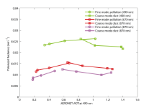
Figure 2 shows the polarized radiances of three PARASOL polarized channels (490, 670, and 865 nm) as a function of AOT. The polarized radiances increased as the AOT increased for fine-mode aerosols. This meets our expectation, i.e., the higher the fine mode AOT, the higher the polarized radiance due to fine mode particles. On the contrary, the polarized radiances at 490 nm and 670 nm decrease as the AOT increases for dust aerosols. This is because of the depolarization effect of irregular coarse dust particles. Thus, spectral variation of polarized radiances with AOT observed by PARASOL can be used to distinguish aerosol types.
 | Figure 2 The polarized radiances at 490, 670, and 870 nm as a function of AOT for coarse-mode dust and fine-mode pollution in Beijing. |
Two other AERONET sites were sampled to get more data. Alta Floresta, located at the southern edge of the Amazon rain forest (9.87°S, 56.10°W), and Maine Soroa, located quite near to the Sahara-Sahel desert (13.22°N, 12.02°E), were selected. Biomass burning aerosols are produced by forest and grassland fires at the Alta Floresta site. The dominant aerosol type is coarse-mode dust particles at the Maine Soroa site. Similar to the study at the Beijing site, fine-mode pollution cases with different AOTs were analyzed from Alta Floresta data, and dust cases with different AOTs were analyzed from Maine Soroa data.
For all cases, the PARASOL pixels of the 200 km × 200 km zone around every site were considered. The scattering angles usually range from ~ 90° to ~ 160° for PARASOL observation geometry. The variation in scattering angle range narrowed down to ~ 100° to ~ 120° for dust days independent of geological location. Measurements at ~ 100°, ~ 105°, ~ 110°, ~ 115°, ~ 120°, ~ 130°, ~ 140°, and ~ 150° scattering angles were used to analyze the spectral ratio of the polarized radiances for five AOT bins. Only the observation samples at the ~ 110° scattering angle were comprehensive enough to generate a useful scatter plot. Therefore, the measurements at ~ 110° (109°< Θ<111°) scattering angle were used. To exclude the effect of aerosol concentration, data were analyzed separately into five AOT bins (0.5-0.6, 0.9-1.1, 1.2-1.3, 1.5-1.75, and 2.0-2.5).
The scatter plots of polarized radiances for the 490 nm and 670 nm wavelength pair for the five AOT bins are shown in Fig. 3. The green triangles and black dots are for fine-mode pollution and coarse-mode dust, respectively. It can be seen that the slopes from linear fits of polarized radiance at 670 nm and 490 nm are less than 0.35 for coarse dust aerosols. However, the slopes for fine-mode aerosols are greater than 0.60. These distinct slopes for coarse- and fine-mode aerosols allow us to use polarized radiance data and variation of polarized radiance with AOT, as described in section 3.1, to classify aerosol types. This is the basis for the SVM feature selection described in section 3.3.
Using the suggestion derived in section 3.2, the PARASOL multi-spectral polarized data and multiclass SVM method were combined to identify four sky conditions (clear, cloudy, fine-mode aerosol pollution, and coarse-mode dust).
A set of features that describes one case (i.e., a row of predictor values) is called a vector feature. Twelve vector features were chosen for this study. They are radiances at 490, 670, and 865 nm; polarized radiances at 490, 670, and 865 nm; spectral ratios of radiance: L(670)/ L(490), L(865)/ L(490), L(865)/ L(670); and spectral ratios of polarized radiance: Lp(670)/ Lp(490), Lp(865)/ Lp(490), Lp(865)/ Lp(670).
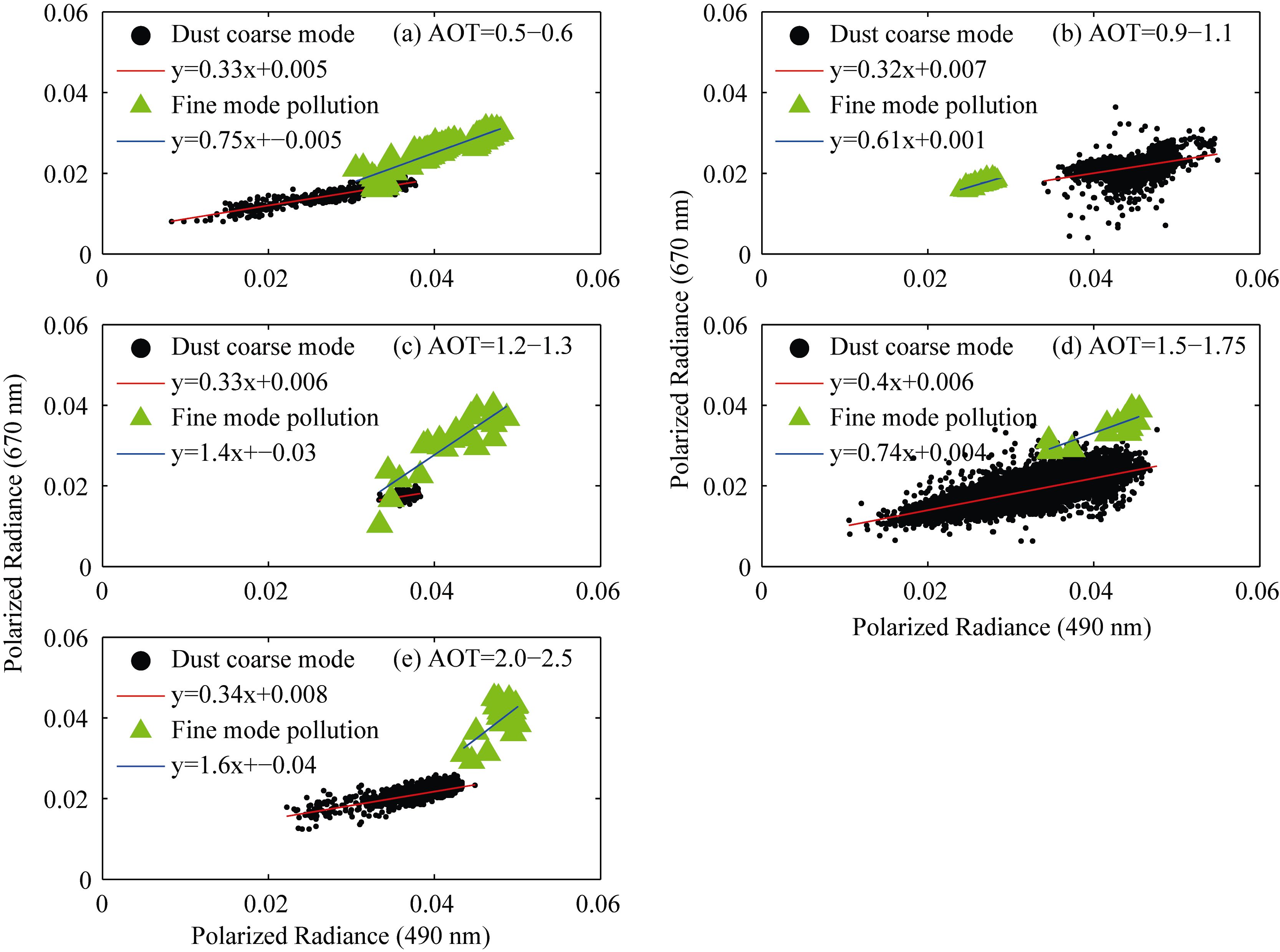 | Figure 3 Scatter plots and linear fits for polarized radiance pairs at 670 and 490 nm for different AOT bins considering fine-mode pollution and coarse-mode dust. |
For the analysis, the training samples were selected according to different sky conditions by using the combined Moderate Resolution Imaging Spectroradiometer (MODIS) Red Green Blue (RGB) images, PARASOL images, and AERONET aerosol data. There were 200 training samples, 50 samples for every sky condition. Then the sky conditions on any day were identified by using the multiclass SVM model. It takes ~ 0.25 s to finish each classification.
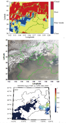
Two specific classification cases are described in thissection. The classification result of fine-mode aerosol pollution on 16 September 2006, around Beijing is shown in Fig. 4a. The corresponding PARASOL RGB image and MODIS/Aqua FMF (Fine Mode Fraction at 550 nm) image are given in Figs. 4b and 4c for comparison. There is good agreement between the classification result and the MODIS FMF image in terms of identifying the aerosol-type regions, although there are some discrepancies in the transitional regions between coarse- and fine-mode aerosols. The smoke plume spreading Beijing-Tianjin-Hebei and Bohai Sea rim region (36-41°N, 114-120°E) in the PARASOL RGB image is obvious in the classification result; however, cloud classification was not accurate. It is possible that since onlyopaque cloud pixels were chosen as the training samples, and translucidus clouds, such as thin cirrus, were not considered, this could have affected the classification results. On 16 September 2006, the ground-based measured AOT at 440 nm, AE (440-870 nm), and FMF at 670 nm from AERONET were 2.06, 1.45, and 0.95, respectively, at the Beijing site. The values at the Xianghe site located between two megacities (Beijing 70 km to the northwest and Tianjin 70 km to the southeast) were 1.92, 1.42, and 0.93. The higher AE (>1.2) and FMF (approaching 1) validated that the fine-mode aerosols were dominant around Beijing that day, which is consistent with the aerosol classification results.
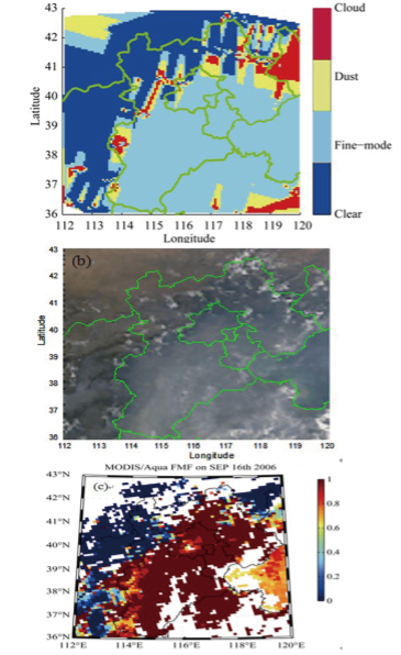 | Figure 4 The classification result using (a) PARASOL data, (b) the PARASOL RGB image, and (c) the MODIS/Aqua FMF (Fine Mode Fraction at 550 nm) image on 16 September 2006 around Beijing. |
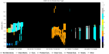
The classification of dust weather on the North China Plain on 24 April 2009, is depicted in Fig. 5a. The corresponding PARASOL RGB image and MODIS/Aqua FMF image are given in Figs. 5b and 5c. The dust plume in the RGB image (Fig. 5b) is consistent with the dust classification results (Fig. 5a). Most MODIS FMF values over the land were less than 0.2, and the rest were less than 0.5. On 24 April 2009, the ground-based measured AOT at 440 nm and AE from AERONET were 1.24 and 0.64, respectively, at the Beijing site. The AERONET measurements were missing for the Xianghe site on that day. The lower AERONET AE (>0.8) and MODIS FMF validated that dust aerosols dominated around Beijing on that day. In addition, the CALIOP (Cloud-Aerosol LIdar with Orthogonal Polarization) VFM (Vertical Feature Mask) aerosol sub-type on 24 April 2009 (Fig. 6), also showed that dust aerosols were spread along the CALIOP orbit ranging from 35.76°N, 116.59°E to 41.15°N, 114.96°E.
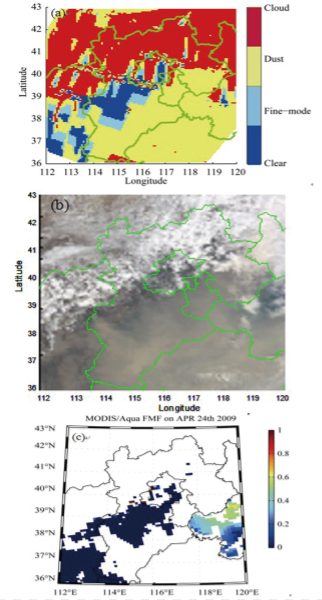 | Figure 5 The classification result using (a) PARASOL data, (b) the PARASOL RGB image, and (c) the MODIS/Aqua FMF image on 24 April 2009 around Beijing. |
There are finely-delineated sky conditions in the RGB image. In comparison, the classification results are relatively rough. A possible reason is that the training samples of SVM were selected and defined according to strictly-delineated sky conditions, taking no account of transitional sky conditions. Furthermore, on the classification images there are straight edges along the regions extending several hundred kilometers. The reason is that classification results are linearly interpolated this surface at the points specified by latitude and longitude. The interpolation has discontinuities in the first and zeroth derivatives, which results in straight line features extending several hundred kilometers. A better interpolation scheme aimed at eliminating these artificial features on classification images will be investigated in a future study.
Another limitation of our classification analysis is that fine- and coarse-mode areas are shown as distinct regions, but in reality, mixed aerosols occur more frequently than regions dominated by just one aerosol, especially around Beijing. However, it is very difficult to detect a mixed aerosol using only PARASOL data, at present. For our next study, we will try detecting mixed aerosols by combining PARASOL, MODIS, and CALIOP data.
 | Figure 6 The Cloud-Aerosol Lidar with Orthogonal Polarization (CALIOP) Vertical Feature Mask (VFM) aerosol sub-type image on 24 April 2009. |
| 1 |
|
| 2 |
|
| 3 |
|
| 4 |
|
| 5 |
|
| 6 |
|
| 7 |
|
| 8 |
|
| 9 |
|
| 10 |
|
| 11 |
|
| 12 |
|
| 13 |
|