 residual
 , or
, or
Slow and Intraseasonal Modes of the Boreal Winter Atmospheric Circulation Simulated by CMIP5 Models
YING Kai-Ran1, 2 , ZHAO Tian-Bao1  , ZHENG Xiao-Gu
2
, ZHENG Xiao-Gu|
|


The authors evaluate the performance of models from Coupled Model Intercomparison Project Phase 5 (CMIP5) in simulating the historical (1951-2000) modes of interannual variability in the seasonal mean Northern Hemisphere (NH) 500 hPa geopotential height during winter (December-January-February, DJF). The analysis is done by using a variance decomposition method, which is suitable for studying patterns of interannual variability arising from intraseasonal variability and slow variability (time scales of a season or longer). Overall, compared with reanalysis data, the spatial structure and variance of the leading modes in the intraseasonal component are generally well reproduced by the CMIP5 models, with few clear differences between the models. However, there are systematic discrepancies among the models in their reproduction of the leading modes in the slow component. These modes include the dominant slow patterns, which can be seen as features of the Pacific-North American pattern, the North Atlantic Oscillation/Arctic Oscillation, and the Western Pacific pattern. An overall score is calculated to quantify how well models reproduce the three leading slow modes of variability. Ten models that reproduce the slow modes of variability relatively well are identified.
Northern Hemisphere atmospheric winter teleconnection patterns and modes of interannual variation have been evaluated over many decades (e.g., Walker and Bliss, 1932; Kutzbach, 1970; Van Loon and Rogers, 1978; Wallace and Gutzler, 1981; Barnston and Livezey, 1987; Frederiksen and Zheng, 2004). There is strong evidence for the existence of a number of important teleconnections, including the Pacific-North American (PNA) pattern, the North Atlantic Oscillation/Arctic Oscillation (NAO/AO), the Western Pacific (WP) pattern, the East Atlantic (EA) pattern, the Tropical Northern Hemisphere (TNH) pattern, the East Atlantic/Western Russia (EA/ WR) pattern (or the Eurasian (EU) pattern), and the Scandinavian (SCA) pattern. The 500 hPa geopotential height is often used to characterize the modes of variability of large-scale atmospheric circulations. Therefore, the ability of coupled atmospheric-ocean general circulation models (CGCMs) to reproduce coherent patterns, or modes, of interannual variability at the 500 hPa geopotential height is an important consideration in the use of such models and in understanding how these modes might change in the future. However, model-simulated heights can be biased and the predictive skill achieved is still not very satisfactory, especially outside of the Tropics ( Zheng et al., 2008).
In the extratropics, a substantial component of interannual variability of seasonal mean fields arises from variability within the season ( Madden, 1981; Zheng and Frederiksen, 1999, 2004; Frederiksen and Zheng, 2000; Zheng et al., 2000). For this reason, it has been referred to as the “intraseasonal component” by Zheng and Frederiksen (2004; hereafter ZF04). This component mainly arises from day-to-day weather variability with time scales longer than the deterministic prediction period (about 10 days) and, therefore, this intraseasonal component is essentially unpredictable on seasonal, or longer, time scales. After removing the intraseasonal component from seasonal mean fields, the residual component is more likely to be associated with slowly varying external forcings (e.g., sea surface temperature (SST)) and from slowly varying (interannual or longer, slower than the intraseasonal time scale) internal atmospheric variability. This residual component is potentially more predictable at the long range ( Madden, 1976). As a result, this component of the seasonal mean fields has been referred to as the “slow component” (ZF04). ZF04 provided a method for estimating, from monthly mean data, spatial patterns of the slow and intraseasonal components. It has been used to identify patterns of the slow and intraseasonal component for the 500 hPa geopotential height field for the Northern Hemisphere (NH) ( Frederiksen and Zheng, 2004; hereafter FZ04) and the Southern Hemisphere (SH) ( Frederiksen and Zheng, 2007a, b), using National Centers for Environmental Predication (NCEP) and National Center for Atmospheric Research (NCAR) reanalysis data. Based on these identified patterns of slow and intraseasonal patterns, Grainger et al. (2013) assessed the models in the Coupled Model Intercomparison Project Phase 3 (CMIP3)
dataset to identify models that reproduced the modes of variability in the SH relatively well and used an ensemble from four models that suitably reproduced the twentieth century modes to examine changes of modes during that time period.
In this study, the modes of interannual variability in the NH 500 hPa geopotential height in CGCMs from Coupled Model Intercomparison Project Phase 5 (CMIP5) dataset ( Taylor et al., 2012) are assessed for the second half of the twentieth century. The modes of variability in the intraseasonal and slow components are compared against those estimated using reanalysis data from the Twentieth Century Reanalysis (20CR) project ( Compo et al., 2011), using the variance decomposition method provided by ZF04. An overall score for quantifying the performance of the CMIP5 models is calculated for each individual model.
The reanalysis monthly mean NH 500 hPa geopotential height used is from the 20CR dataset for the period 1951- 2000. The 20CR project uses a recent AGCM and data assimilation system to generate an ensemble of forecasts of the atmospheric circulation using only surface pressure observations and monthly SST and sea-ice measurements. Although satellite data are not used, the quality of the 20CR dataset is at least comparable to other reanalysis products (e.g., Compo et al., 2011; Stachnik and Schumacher, 2011). For the modes of variability of the slow component, we are also interested in their relationship with the global SST. The SST data used are from the HadISST dataset ( Rayner et al., 2003).
The monthly mean 500 hPa geopotential height from the CMIP5 dataset was obtained for the last 50 years of the historical experiment. For assessment of the modes of variability of the intraseasonal and slow components, 86 historical realizations from 26 models used in this study are summarized in Table 1. Surface skin temperature data over oceans are used to represent model SST.
To compare the CMIP5 models with reanalysis data, all 500 hPa geopotential height data are mapped onto the same 2.5° ´ 2.5° longitude/latitude grid, then sub-sampled to 5° ´ 5°. This is thinned towards the North Pole, as in FZ04, so that the data are approximately weighted by area. All SST data are mapped onto the same 2° ´ 2° latitude/longitude grid. Before analysis, the annual cycle is removed by subtracting the climatological monthly mean for 1951-2000.
ZF04 proposed a methodology for extracting, from monthly mean data, spatial patterns of interannual (supra- annual) variability in seasonal mean fields related to the variability of slow and intraseasonal components ( Frederiksen and Zheng, 2007b). Here, we present only a brief summary of the method.
First, the annual cycle is removed from the monthly time series. The monthly anomaly is then conceptually decomposed into two components consisting of a seasonal “population” mean and a residual departure from this population mean. Thus, if xym represents sample monthly values, within a season, in month ( m = 1, 2, 3) in year ( y = 1,…., Y, where Y is the total number of years), we use the following decomposition (for reference, see ZF04): 
Here, μy is the seasonal population mean in year yand εym is a residual monthly departure of xym from μy. The vector { εy1, εy2, εy3} is assumed to comprise a stationary and independent annual random vector with respect to the year. Equation (1) implies that month-to-month fluctuations, or intraseasonal variability, arise entirely from { εy1, εy2, εy3} (e.g., ( xy1? xy2= εy1? εy2)).
We represent an average taken over an independent variable (i.e., m or y) by replacing that variable subscript with “ o”. With this notation, a seasonal mean can be expressed as
 | , (2) |
where εyo is associated with the intraseasonal variability and μy is associated with the interannual variability of external forcing and slowly varying (interannual/supra- annual) internal dynamics.
Given monthly mean anomalies, ZF04 showed that interannual covariance matrices for the components of the seasonal mean can be estimated. Once the intraseasonal and residual covariance matrices have been estimated, a varimax rotated empirical orthogonal function (REOF) (weighted with the square root of the eigenvalues of the covariance matrix) analysis is conducted to identify the leading intraseasonal and slow modes of each covariance matrix, respectively, to get the slow modes of variability (S-REOFs) and intraseasonal modes of variability (I- REOFs).
For S-REOFs, the relationship with SST is considered using the covariance between the slow component in both the associated time series of the S-REOF and SST time series. This is calculated at each SST grid point using the methodology of Grainger et al. (2011a), and is described here as the slow SST-height covariance.
Since all 500 hPa geopotential height and SST data have been mapped to the same grid, the variances of the REOFs (i.e., the eigenvalues) are directly comparable and pattern correlations of the structures can be calculated ( Grainger et al., 2008, 2013). Based on the principles of Taylor (2001), scores for how well a model reproduces a 20CR slow mode of interannual variability can then be defined as REOFs, R is the pattern correlation between the model and 20CR S-REOFs (the absolute value is used since the sign of a REOF is arbitrary), and RSST is the pattern correlation, over a given region, between the structures of the model and 20CR SST time series related to the S-REOFs. This relationship is defined as the slow covariance between the associated time series of the S-REOFs and the SST time series at each grid point, and is estimated using the methodology of Grainger et al. (2011a).
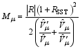 | , (3) |
where 

| Table 1 CMIP5 models and the number of historical realizations used in this study. |
An overall score is defined for each model ensemble, or individual realization, as
 | , (4) |
where ( Mμ) n is the score estimated from Eq. (3) for the model “best match” (details can be found in Grainger et al. (2013)) to the 20CR S-REOFs, Nis the number of the S-REOFs we evaluated.
The leading nine I-REOFs of the NH December-January-February (DJF) 500 hPa geopotential height for the 20CR reanalysis explained 84% of the interannual covariance in total (figures not shown here). Qualitatively, the 20CR intraseasonal modes are similar to those estimated using NCEP reanalysis data for the period from 1958 through 1996 (Fig. 3 in FZ04), although the estimated variances of these patterns vary slightly. These are patterns that are related to intraseasonal variability in the PNA, EA, EA/WR, TNH, and SCA patterns as well as Greenland, West Pacific, and Alaskan blocking.
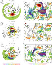
Since the leading three 20CR S-REOFs explain 67% of the covariance of the slow component in DJF, we investigate how well the patterns of the observed slow component are simulated by the CMIP5 multi-models, considering these three leading modes. The leading three S- REOFs of the NH DJF 500 hPa geopotential height for 20CR reanalysis and its associated slow SST-height covariance with the HadISST SST are shown in Fig. 1. The patterns have horizontal structures and SST relationships similar to those observed in FZ04. In particular, features of the PNA, NAM, and WP patterns could be seen in the first three modes, with high correlations to ENSO, the North Atlantic triple pole, and SSTs in the Indian Ocean and the northwestern Pacific at 0-season lag, respectively. There is a much clearer separation between the variance explained by S-REOF1 and S-REOF2 in the 20CR than in the NCEP reanalysis (Fig. 4 in FZ04). The NCEP reanalysis S-REOFs have higher estimated standard deviations (Table 4 in FZ04) than the 20CR, particularly for S-REOF1. Bromwich and Fogt (2004) found that the NCEP reanalysis has a bias and an artificial linear trend at high latitudes. It is possible that this may result in higher estimates of the interannual covariance. The ability for CMIP5 multi-models to reproduce the structure of the S-REOFs, the structure of the slow SST-height covariance, and to estimate the associated variance will be discussed separately in the following sections. An overall score for the CMIP5 assessment is based on the above three factors.
Firstly, we examined how well the leading nine I- REOFs were simulated by the CMIP5 models (figures not shown). For individual CMIP5 models, the spatial structures of the leading nine I-REOFs are very similar to the 20CR reanalysis with spatial correlations averaged to ~ 0.8. Although these modes are generally present, they are not necessarily in the same order as the 20CR; specifically, the model mode that best reproduces the 20CR I-REOF1 may not be the I-REOF1 in the CMIP5 models. However, the explained variances for the dominant nine modes do not have too many differences. So the leading modes of variability in the intraseasonal component are generally well reproduced by the CMIP5 models.
The ability of the CMIP5 models to reproduce the leading three 20CR S-REOFs is summarized in Fig. 2. The pattern correlations for S-REOFs (| R|) and slow SST- height covariances ( RSST), as well as the relative standard deviation, are calculated between the CMIP5 models and 20CR. Here, the regions chosen to evaluate RSST are the regions of high slow SST-height covariance seen in Figs. 1d-f, as we have discussed and summarized in the previous section. In particular, RSST is calculated over the region 20°S-40°N for S-REOF1; 0°N-50°N and 270°E- 360°E for S-REOF2; and 0°N-40°N and 60°E-120°W for S-REOF3.
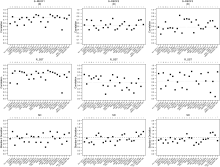
 | Figure 2 For the CMIP5 models: the REOF pattern correlation | R| (top panels), the pattern correlation between the slow SST-height covariance, RSST(middle panels), calculated over the region 20°S-40°N for S-REOF1; 0°N-50°N and 270°E-360°E for S-REOF2; and 0°N-40°N and 60°E-120°W for S-REOF3, the relative standard deviation (SD) (bottom panels), to the 20CR DJF S-REOFs. For each model, the median over the ensemble estimate is shown by the dashed line. The number of realizations for each model is given above the plot. |
For S-REOF1 (left column of Fig. 2), the values of | R| and RSST are high across most of the models, with the median ensemble value of about 0.78 and 0.75, respectively. The highest values of | R| are found in HadGEM2-ES, IPSL-CM5A-LR, NorESM1-M, ACCESS1-0, and NorESM1-ME, while inmcm4 stands out as having the lowest pattern correlations. Models that reproduce the spatial structure of modes relatively well are more likely to have above-median values of RSST. There is a wide range of values of relative standard deviations, although the median is close to 1.0; MIROC-ESM, CNRM-CM5, and inmcm4 have particularly low values and reproduce the 20CR S-REOF1 relatively poorly.
For S-REOF2 (middle column of Fig. 2), the median ensemble values for | R| and RSST are about 0.52 and 0.48, respectively. This is much lower than for S-REOF1. However, IPSL-CM5A-LR, GFDL-ESM2G, MIROC-ESM- CHEM, CSIRO-MK3-6-0, and IPSL-CM5A-MR reproduce the REOF spatial structures relatively well. They also have above-median values of RSST. This mode is often represented by a higher order S-REOF in the modes. Consequently, the majority of models have magnitudes of relative standard deviations that are lower than 1.0, particularly for MIROC4h and FGOALS-g2, which have values lower than 0.6.
For S-REOF3 (right column of Fig. 2), values of 
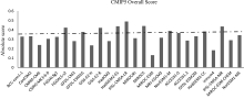
It is useful to quantify how well models reproduce the modes of variability overall in the twentieth century and to identify differences between models. In the previous section, we found that the CMIP5 models considered here generally reproduce well the modes of variability of the intraseasonal component of the NH 500 hPa geopotential height. However, there are clear differences between models as to how well they reproduce the 20CR S- REOFs. So our focus will be on S-REOFs. For this purpose, we define an overall score for each model by Eq. (4) and results are shown in Fig. 3. It can be seen that ten models reproduce the 20CR leading three S-REOFs relatively well, with overall scores well “above median”: IPSL-CM5A-LR, HadGEM2-ES, MIROC5, FGOALS-s2, IPSL-CM5A-MR, GISS-E2-R, GFDL-ESM2G, NorESM1- M, HadGEM2-CC, and ACCESS1-0. The results are consistent with discussions about the CMIP5 model performances in the previous section.
In this paper, modes of interannual variability in the slow and intraseasonal component of the seasonal mean NH DJF 500 hPa geopotential height were estimated based on the CMIP5 multi-model simulations. Modes of variability in the components were assessed against those estimated using the 20CR reanalysis. To evaluate the performance of individual models, the spatial structure and variance of the model modes of variability in the slow component, as well as their relationships with SST, were assessed. Also, an overall score was given to quantify how well models reproduce modes of variability in 20CR. Our key findings are:(1) The leading nine modes of variability in the intraseasonal component are generally well reproduced in the CMIP5 models, with few clear differences between models.
 | Figure 1 (a-c) The leading three slow REOFs (rotated empirical orthogonal function) of the 20CR NH (Northern Hemisphere) 500 hPa geopotential height for DJF 1951-2000. (d-f) Slow SST-height covariance with HadISST (The Hadley Centre Global Sea Ice and Sea Surface Temperature) for the leading three slow REOFs. The estimated standard deviation (m) and variance explained (%) are given to the left of each REOF. |
(2) There are clear differences between models in their reproduction of the leading three modes of variability in the slow component. These include the dominant slow patterns in the NH, i.e., the PNA, the NAO/AO, and the WP patterns. Overall, the slow patterns are not as well simulated. Only PNA is captured well both in the spatial pattern and SST-height covariance pattern. For the remaining two slow modes, the spatial patterns cannot be reasonably well captured by most of the CMIP5 models.
 | Figure 3 Absolute overall score for the CMIP5 models calculated using the ensemble estimates. The median value of the overall scores is shown by the dashed lines. |
(3) An overall score is calculated using the leading three modes of variability in the slow component. Clear differences were found between the CMIP5 models, and ten models were identified as relatively better able to reproduce modes of variability in 20CR, with “above median” overall scores: IPSL-CM5A-LR, HadGEM2-ES, MIROC5, FGOALS-s2, IPSL-CM5A-MR, GISS-E2-R, GFDL-ESM2G, NorESM1-M, HadGEM2-CC, and ACCESS1-0.
We hypothesize that the main reason that the models are better at simulating the intraseasonal modes is because this only requires that the model dynamics be good. The models' "dynamical core" is generally pretty good because it is basically just F = m • a; however, the slow modes require that the "physics code" (i.e., the radiation code, cloud schemes, and boundary layer parameterizations) also be good and this varies from model to model, depending on the physical parameterizations being used. The model physics is the area in which the models generally have their largest sources of error. Additionally, in coupled models the atmosphere-ocean interaction is important, and this is generally another area where the models lack skill.
In future work, how the modes of interannual variability are projected to change in the CMIP5 Representative Concentration Pathways (RCP) experiments will be examined, using an ensemble from the models that suitably reproduces the twentieth century modes of variability that we have identified in this work.
| 1 |
|
| 2 |
|
| 3 |
|
| 4 |
|
| 5 |
|
| 6 |
|
| 7 |
|
| 8 |
|
| 9 |
|
| 10 |
|
| 11 |
|
| 12 |
|
| 13 |
|
| 14 |
|
| 15 |
|
| 16 |
|
| 17 |
|
| 18 |
|
| 19 |
|
| 20 |
|
| 21 |
|
| 22 |
|
| 23 |
|
| 24 |
|