Optimal Precursor Perturbations of El Niño in the Zebiak-Cane Model for Different Cost Functions
Optimal Precursor Perturbations of El Niño in the Zebiak-Cane Model for Different Cost Functions |
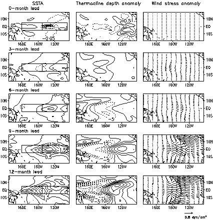
| Figure 5 The evolution patterns of the optimal precursor with initial time October and lead times 3, 6, 9, and 12 months for the cost function defined as the SSTA development in the Ni#cod#x000f1;o4 area. The left column is the SSTA component, the middle column is the thermocline depth anomaly component, and the right column is the corresponding wind stress anomalies. The square frames label the Ni#cod#x000f1;o3 and Ni#cod#x000f1;o4 areas. The contour interval is 0.05#cod#x000b0;C for 0-month lead SSTA, 0.5#cod#x000b0;C for other SSTA, 0.5 m for 0-month lead thermocline depth anomaly, and 5.0 m for others. |
| |