An Extension of the Dimension-Reduced Projection 4DVar
Cite this Article
SHEN Si, LIU Juan-Juan, WANG Bin. An Extension of the Dimension-Reduced Projection 4DVar. Atmospheric and Oceanic Science Letters, 2014, 7(4): 324-329 
Permissions
Copyright?2014, Editorial office of Atmospheric and Oceanic Science Letters
This is an Open Access article under the terms of CCAL.
An Extension of the Dimension-Reduced Projection 4DVar
Abstract
This paper extends the dimension-reduced pro-jection four-dimensional variational assimilation method (DRP-4DVar) by adding a nonlinear correction process, thereby forming the DRP-4DVar with a nonlinear correction, which shall hereafter be referred to as the NC-DRP- 4DVar. A preliminary test is conducted using the Lor-enz-96 model in one single-window experiment and several multiple-window experiments. The results of the single-window experiment show that compared with the adjoint-based traditional 4DVar, the final convergence of the cost function for the NC-DRP-4DVar is almost the same as that using the traditional 4DVar, but with much less computation. Furthermore, the 30-window assimilation experiments demonstrate that the NC-DRP-4DVar can all-eviate the linearity approximation error and reduce the root mean square error significantly.
Keyword:
data assimilation; linear approximation; non-linear correction; OSSE
Received 6 November 2013; revised 28 January 2014; accepted 19 February 2014; published 16 July 2014
Citation: Shen, S., J.-J. Liu, and B. Wang, 2014: An ext-en-sion of the dimension-reduced projection 4DVar, A t mos. Oce - anic Sci. Lett., 7, 324-329, doi:10.3878/j. issn.1674-2834.13.0087.
1 Introduction
One of the important strategies of improving the operational implementation of 4DVar is to develop an ensemble-based 4DVar (En4DVar), which uses an ensemble met-hod similar to the one used in the ensemble Kalman filter (EnKF) for obtaining a solution for the minimization of 4DVar. En4DVar includes almost all the advantages of both standard 4DVar and EnKF. In recent years, there have been some efforts in the development of the En4DVar family ( Lorenc, 2003; Qiu et al., 2007; Cao et al., 2007; Liu et al., 2008; Tian et al., 2008; Wang and Li, 2009; Wang et al., 2010; Liu et al., 2011; Tian et al., 2011). The dimension-reduced projection 4DVar (DRP-4DVar) pro-posed by Wang et al. (2010) is one of the representative approaches of this family.
The DRP-4DVar solves the 4DVar problem in the subspace defined by an ensemble. This approach conserves the advantages of the 4DVar while avoiding the use of the adjoint model. Besides, similar to the EnKF, it uses real- time ensemble to estimate the background error covariance outside the assimilation window. An idealized model experiment using the Lorenz-96 model ( Liu et al., 2011) shows that DRP-4DVar outperforms the EnKF, which benefits from the inclusion of model constraints in DRP- 4DVar. Its performances are also verified by real models such as the Penn State/National Center for Atmospheric Research (NCAR) fifth generation mesoscale model (MM5) (e.g., Wang et al., 2010; Zhao et al., 2012). However, like many other ensemble-based methods, some aspects of the DRP-4DVar require further improvements and developments, one of which is the further reduction of its cost function. In DRP-4DVar, a linear approximation is made to simplify its solution, which however may cause extra errors in the analysis and limit the reduction of cost function.
To deal with this, this paper presents an iterative non-linear correction process for DRP-4DVar. This iterative nonlinear correction process is inspired by the incremental approach, which was first proposed by Courtier et al. (1994) for the operational implementation of the 4DVar ( Courtier et al., 1994 , Courtier and Andersoon, 1998; Hu-ang et al., 2009). It divided the original cost function into a sequence of simplified cost functions. Thus, the minimi-zation procedure was divided into a pair of nested loops, that is, the outer and inner loops. The outer loop iteration updated the model of "state of the art", while the inner loop performed iterative minimization on the reduced- resolution model and the result of the inner loop was used to prepare for the next outer loop iteration. In this case, the tangent linear model and adjoint model for the 4DVar were of a lower resolution so that the computational cost could be largely reduced. From this "outer & inner loop" idea, a similar extension is made for the DRP-4DVar. In this extension, the original DRP-4DVar, which is solved directly and easily but with linear approximation, is tre-ated as a special inner loop. In the outer loop, the background and the ensemble are updated by the nonlinear model to refine the results from the inner loop iteratively. This extended version of DRP-4DVar is hereafter referred to as the DRP-4DVar with a nonlinear correction (or NC- DRP-4DVar as an acronym).
This paper is organized as follows. The basic principle of the NC-DRP-4DVar is described in section 2 and the preliminary test is dealt with in section 3. Finally, the summary and discussion are provided in section 4.
2 Methodology
2.1 A brief review of the DRP-4DVar
4DVar produces an optimal analysis by minimizing the cost function:
| , (1) |
where the superscript T denotes the transpose, the bold- faced variables represent the column vectors or matrices, the argument x0 is the analysis in the L x-dimensional model space with its time being in the beginning of the assimilation window, x0b is its background, and the ( L x× L x) dimensional matrix B is the background error covariance. The letter Y (in upper case) represents an observation vector of dimension L y containing all observations within the observation window, while the letter y (in lower case) represents an observation vector at a single time, i.e., { y i } are subvectors of Y. Yo is the observation vector and Y( x0) is the simulated observation vector. N is the total number of observation times within the assimilation window, ( t1, t2, ...., t N) are the times of observations, H i is the observation operator at time t i, M t0 →ti is the forecast model integration from t0(the beginning of the window) to t i , and O is the observation error covariance matrix of dimension ( L y× L y). The circle symbol
If we have an ensemble of initial condition perturbations P x given by
| , (2) |
and if the analysis (a) increment can be expressed as a linear combination of the ensemble members as
| , (3) |
where
| , (4) |
where
From Eqs. (1), (2), (3), and (4), the cost function of 4DVar can be rewritten as a function of
| (5) |
From the definition of
| , (6) |
where
| (7) |
With the inverse of
2.2 A brief review of the incremental approach
Before presenting the NC-DRP-4DVar let us briefly review the main idea of the incremental approach. The original 4DVar cost function (Eq. (1)) is complex and fully- nonlinear and its solution needs many iterations. For each iteration, at least one nonlinear model integration and one adjoint model integration are needed. Thus, 4DVar is an intensive computational method. In order to simplify the solution and reduce the computational cost, Courtier et al. (1994) proposed a linear approximation in terms of inc-rements, which is valid in the vicinity of x0b, as follows:
| , (9) |
where the operator
| (10) |
The inner loop solves the quadratic J i iteratively while the outer loop updates J i using the results
2.3 The DRP-4DVar with a nonlinear correction
As shown in section 2.1, a linear approximation is used in Eq. (6). It is necessary for the minimization process of the DRP-4DVar. However, the approximation leads to our analysis being suboptimal, especially when the observation operator or the model has strong nonlinearity or the analysis increment
Similar to Eq. (10), NC-DRP-4DVar divides Eq. (5) (or its equivalence, Eq. (5')) into a list of quadratic cost functions as given by Eq. (11) below.
| , (11) |
where the operator
3 Experiments and results
3.1 Basic description of the experimental design
The observing system simulation experiment (OSSE) is considered to be one of the best choices for evaluating data assimilation schemes. As a preliminary test, we use the Lorenz-96 model ( Lorenz, 1996) to perform the OSSE:
| , (12) |
where j=1, 2,..., M , represents the spatial coordinates and the system satisfies the periodic boundary condition, i.e.,
Here, we are only concerned about the observation term as it is the source of linear approximation errors; therefore, the background term is ignored for simplicity. Since no error correlation exists between observations, the cost function to test here is simplified as
| , (13) |
where the tilde (~) above Y indicates that it has been normalized by the observation error standard deviation, i.e.,
| (14) |
and the form
For both DRP-4DVar and NC-DRP-4DVar, the ensemble
The ensemble updating strategy
This strategy is theoretically reasonable but requires large computation. A simpler strategy is presented here, which is a "no-updating strategy" given as
| (16) |
This strategy is empirical but needs no extra computation and thus is very efficient and worth testing. In this paper, hereafter, NC-DRP-4DVar is based on this strategy, unless otherwise stated.
As a reference, the traditional 4DVar using the adjoint model is also performed and solved by the incremental approach, as shown in section 2.2 but no resolution reduction is used in the inner loop. The number of outer loop iterations is also set to 5 and the inner loop is solved by the conjugate gradient method and it terminates when there is a 90% reduction in the norm of the cost function gradient. The cost function of the traditional 4DVar is also simplified for comparison as follows:
| (17) |
3.2 Single-window experiment
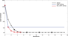
A single-window assimilation experiment is carried out to demonstrate the decrease of cost function due to the nonlinear correction for the DRP-4DVar. The variation of the NC-DRP-4DVar and 4DVar cost function values during iterations is shown in Fig. 1. Besides, the cost function variation of DRP-4DVar is also shown in the figure as it can be seen as the NC-DRP-4DVar converging after one outer loop. As shown in Fig. 1, the final convergence value of the NC-DRP-4DVar cost function is almost the same as that of 4DVar. From this it may be concluded that the isolation of linear approximation error of the DRP- 4DVar is successful, otherwise the NC-DRP-4DVar cost function can't achieve the comparable convergence with 4DVar. Compared to DRP-4DVar, there is a 40% decrease in the cost function of NC-DRP-4DVar, suggesting a significant improvement due to the nonlinear correction process. This large decrease in magnitude also suggests that the effect of linear approximation is significant even with linear observations.
 | Figure 1 Variation of cost function values of 4DVar (black curve), DRP-4DVar (blue curve), and NC-DRP-4DVar (red curve) during iterations. X-coordinate represents iterations and Y-coordinate represents cost function value in a logarithmic scale. Circles along curves represent outer loop iterations of 4DVar or NC-DRP-4DVar. Triangles along curves represent inner loop iterations of 4DVar. |
Considering the computational cost, NC-DRP-4DVar only needs about four iterations to converge and for each iteration only one nonlinear model integration is required, while for 4DVar convergence occurs after about eight inner iterations (in the 3rd outer loop iteration) with at least one tangent linear model integration and one adjoint model integration required for each inner loop iteration and one extra nonlinear model integration required for each outer loop iteration. As we know, the cost of adjoint model integration is about five to eight times higher than that for nonlinear model integration. Thus, though this extension of DRP-4DVar increases its computational cost, it is still much less than that for the traditional 4DVar.
3.3 Multiple-window experiments
To test the overall performance of the NC-DRP-4DVar in a longer time, a multiple-window assimilation experiment consisting of 30 windows is conducted. As each window length is of 18 h, the assimilations take place every 24 h and a total of 30 days (120 steps) integration is required. A control run (namely CTRL) starts with the background at the initial time and integrates for 30 days without assimilation. The CTRL run provides the back-
ground field for assimilation schemes in every window. Four assimilation schemes including the above mentioned 4DVar, DRP-4DVar, NC-DRP-4DVar, and an extra NC- DRP-4DVar scheme using the 're-integrating' updating strategy given in Eq. (15), namely NC-DRP-4DVar_RI, are conducted.
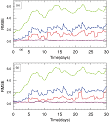
Figure 2a shows the root mean square errors (RMSEs) of the background (CTRL) and analyses from the four schemes. It should be noted that here the ensemble P x is regenerated independently for each window, and the back-
ground term in the cost function is ignored; hence, some of their advantages such as the explicitly flow-dependent background covariance versus the fixed background cov-ariance in the traditional 4DVar cannot be shown. So it is unfair to evaluate the DRP-4DVar related schemes simply by comparing them with the 4DVar in this situation. How-ever, if we are only concerned about the nonlinear effect, the 4DVar here can be treated as a reference.
As shown in Fig. 2a, the RMSE of 4DVar maintains a
 | Figure 2 RMSEs of CTRL (green dashed), 4DVar(black solid), DRP- 4DVar (blue dashed), NC-DRP-4DVar (red dashed), NC-DRP-4DVar_ RI (pink dashed, overlapping with the black solid 4DVar) during 30 days for (a) full observations and (b) observations available at time 0/3. |
very low and nearly constant level during the 30-day assimilation. It is because no background term is contained in the cost function (Eq. (17)) and thus the background should have no impact on the analysis theoretically. However, for DRP-4DVar, its large-valued RMSE increases along with the increase in the background RMSE apparently, which is different from the theoretical fact mentioned above. This can be attributed to the linearity approximation in its solution. If the background is inadequately provided, the analysis increments
Besides these experiments, a cycling assimilation experiment is also conducted. Instead of using CTRL as background, the cycling assimilation experiment uses the forecast of the analysis from the last window as its background. For long-time integration, all the four schemes perform well and the RMSEs (not shown) are almost the same after several cycles. It is inferred that under the idealized conditions (perfect model, sufficient, and linear observations, etc.), all the assimilation schemes work well so that the backgrounds are all of good quality. In this case, the linear approximation is reasonable and much smaller errors are introduced.
4 Summary and conclusions
Many ensemble-based variational assimilation methods try to avoid the use of the adjoint model by using an explicit quadratic cost function and then solving it directly, which may introduce errors caused by linear approximation and limit the reduction of the cost function. Here, the idea of the incremental approach to introduce the nonlinear effect iteratively is adopted to further reduce the cost function in the DRP-4DVar, forming the DRP-4DVar with a nonlinear correction (NC-DRP-4DVar). In the implementation of the NC-DRP-4DVar, two strategies to update the ensemble are introduced: one is the theoretically correct but time consuming 're-integrating' strategy which needs to integrate all members of the ensemble for each outer loop iteration and the other one is an empirical and economical 'no-updating' strategy in which no ensemble updates.
The preliminary test using the Lorenz-96 model, gridded observations, and a simplified cost function without the background term is conducted. One single-window experiment is carried out and the result shows perfect convergence of the cost function for the NC-DRP-4DVar, i.e., a further decrease of 40% over DRP-4DVar and almost the same with the 4DVar. Considering the high com-putation cost of the adjoint model, the NC-DRP-4DVar is still an economical choice compared to the 4DVar. Two kinds of 30-window experiments are carried out; in one the background from the control run is used while the ot-her is a cycling assimilation experiment. In the first case in which the background is poor and hence the nonlinearity effect is strong, great improvement is shown, especially when using the 're-integrating' updating strategy. In spite of this, the RMSE reduction of the other economical scheme (i.e., using the 'no-updating' strategy) is also impressive. In the second case in which the background is of good quality, all the assimilation schemes perform perfectly as a result of weak nonlinearity. The results of all these experiments indicate a significant improvement of the NC-DRP-4DVar and convince us to investigate further.
In real situations, both the model and the observations may have a much stronger nonlinearity. This nonlinear correction extension for DRP-4DVar is expected to be of more practical help. However, the number of ensembles is limited in real cases and thus techniques including covariance inflation and localization are necessary. Besides, methods of generating sufficient and representative samples remain a key point for the assimilation performance. More investigations of NC-DRP-4Dvar on real cases are necessary before it can be further applied.
Acknowledgements. This work was jointly supported by the National Basic Research Program of China (973 Program, Grant No. 2010CB951604), the National Key Technologies Research and Development Program of China (Grant No. 2012BAC22B02), and the National Natural Science Foundation of China (Grant No. 41105120).
Reference
| 1 |
|
| 2 |
|
| 3 |
|
| 4 |
|
| 5 |
|
| 6 |
|
| 7 |
|
| 8 |
|
| 9 |
|
| 10 |
|
| 11 |
|
| 12 |
|
| 13 |
|
| 14 |
|
| 15 |
|
| 16 |
|