Effect of Decadal Changes in Air-Sea Interaction on the Climate Mean State over the Tropical Pacific
[FANG Xiang-Hui1, 2 , ZHENG Fei1, *  ]
]
]
|
|


Collaboration of interannual variabilities and the climate mean state determines the type of El Niño. Recent studies highlight the impact of a La Niña-like mean state change, which acts to suppress the convection and low-level convergence over the central Pacific, on the predominance of central Pacific (CP) El Niño in the most recent decade. However, how interannual variabilities affect the climate mean state has been less thoroughly investigated. Using a linear shallow-water model, the effect of decadal changes of air-sea interaction on the two types of El Niño and the climate mean state over the tropical Pacific is examined. It is demonstrated that the predominance of the eastern Pacific (EP) and CP El Niño is dominated mainly by relationships between anomalous wind stresses and sea surface temperature (SST). Further-more, changes between air-sea interactions from 1980-98 to 1999-2011 prompted the generation of the La Niña- like pattern, which is similar to the background change in the most recent decade.
El Niño-Southern Oscillation (ENSO), being the most striking large-scale interannual variability originating in the tropical Pacific, has profound influences on the global climate. Although investigated for several decades, ENSO is still far from completely understood, especially given that a new type of El Niño was identified recently. Maximum sea surface temperature (SST) anomalies of this new type of El Niño are concentrated in the central Pacific, and have different effects on global climate ( Kim et al., 2009; Yu et al., 2012). It is referred to as the central Pacific (CP) El Niño ( Yu and Kao, 2007; Kao and Yu, 2009), while the canonical El Niño, which has its maximum warming anomalies located in the eastern Pacific, is referred to as the eastern Pacific (EP) El Niño. Recently, many studies have focused on the frequent occurrences of CP El Niño in the most recent decade (e.g., Yeh et al., 2009; McPhaden et al., 2011; Xiang et al., 2012), arguing this feature is likely due to a mean state change ( Xiang et al., 2012). The past decade has a dramatic La Niña-like mean state pattern when compared to the preceding period: for example, sea surface cooling is apparent in the central and eastern Pacific and warming in the west, extending into the tropics; sea surface height (SSH), which is approximately proportional to thermocline depth, shows a declining trend in the eastern Pacific and a rising trend in the west; excessive easterly wind occurs in the central and western Pacific, while westerly wind occurs in the east; and less precipitation appears over the central Pacific, while more precipitation is observed over the far west. Xiang et al. (2012) argued that such changes of the mean state in the Pacific prompt the generation of CP El Niño through suppressing the convection and low-level convergence in the central Pacific, which highlights influences of the climate mean state on interannual variabilities.
However, the asymmetry of interannual variabilities can also modulate the mean state conditions, but this mechanism has been less investigated (e.g., Jin et al., 2003; Kug et al., 2009; Lee and McPhaden, 2010). Jin et al. (2003) pointed out that changing ENSO is responsible for the significant change of nonlinear heating in the equatorial Pacific, and thus the linear trend in the climate mean state; Kug et al. (2009) argued that the frequent occurrences of CP El Niño contribute to an accumulative warming of the mean state; and Lee and McPhaden (2010) suggested that the warming trend in the Niño4 region is primarily a consequence of more intense and frequent CP El Niño events. This study, following this viewpoint, investigates how decadal changes of air-sea interactions in the past three decades impact the mean state over the tropical Pacific.
All data used in this study cover the period from 1980 to 2011. The SST data are from ERSST (National Oceanic and Atmospheric Administration Extended Reconstructed SST), v3b ( Smith et al., 2008), with a horizontal resolution of 2° × 2°; the SSH data are from National Centers for Environmental Prediction/Department of Energy Global Ocean Data Assimilation System (NCEP GODAS, http://www.esrl.noaa.gov/psd/data/gridded/data.godas.html), with a horizontal resolution of 1° × (1/3)°; and the wind stress data were constructed from European Center Hamburg Atmospheric Model, version 4.5 (ECHAM4.5) ensemble simulations and observed SST via a singular value decomposition (SVD) analysis for the period 1963-96 ( Zheng et al., 2009), with a horizontal resolution of 2° × 2°. To illustrate the decadal changes, the whole analysis period is separated into two sub-periods, i.e., 1980-98 and 1999-2011, as operated in Xiang et al. (2012). Furthermore, to eliminate contamination of the mean state change, the anomalies are all calculated by subtracting the whole climatology.
The model used in this study is a linear coupled model of the equatorial Pacific, GMODEL version 3.0 ( Burgers et al., 2002). Its dynamical model is a linear shallow water ('1.5 layer') model with the only dynamical field being the thermocline depth. The SST model ( Kleeman, 1993), which is valid only in the central and eastern equatorial Pacific, consists of three linear terms: linear damping; a forcing proportional to the thermocline depth anomaly (i.e., thermocline feedback); and a forcing proportional to the zonal wind stress anomaly (i.e., Ekman pumping feedback).
Being the most important and strongly coupled variables of the atmosphere and ocean, wind stress and SST (specifically, Niño3 and Niño4 SST indices) are used to construct the regression relationships to represent the interannual air-sea interactions over the tropical Pacific, i.e.,
ression coefficients; and noise is the Gaussian white and red noise. These statistical relationships are constructed during each sub-period based on the observed datasets. In each integrating step of the experiments, wind stress anomalies are calculated with the updated Niño3 and Niño4 indices, and then force the model to move on. In this study, each experiment is integrated for 100 years.
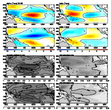
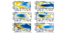
Figure 1 shows the spatial patterns of the coefficients of the regression relationships in 1980-98. For quantitative comparison, the coefficients are multiplied by their corresponding standard deviations of the Niño indices. It can be seen that the major positive coefficients of zonal wind stress anomalies are quite consistent with their respective Niño regions, i.e., positive alphas are mainly located in the Niño3 region (5°S-5°N; 150-90°W), and positive betas are mainly located in the Niño4 region (5°S-5°N; 160°E-150°W). It also shows that the magnitudes of alphas and betas are comparable, indicating that the anomalous zonal wind stresses in this sub-period depend on the SST in both Niño regions. The meridional wind stress anomalies are mainly dominated by the Niño3 index, with large negative coefficients north of the equator and positive ones south of the equator. To assess how well the regression relationships can capture the interannual air-sea interactions, Fig. 1 also shows the correlation coefficients and root-mean-square errors (RMSE) between the regressed wind stresses, which are calculated by the observational Niño indices, and the original wind stress datasets. Large correlation coefficients and small RMSEs are seen to take over most of the tropical regions, especially near the equator. This verifies the appropriateness of the regression relationships constructed by this method.
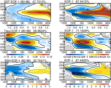
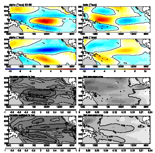
Next, the regression relationships are embedded in the GMODEL to examine what patterns will prevail, and this experiment is named Exp1. The leading empirical orthogonal function (EOF) patterns of anomalous SST, zonal wind stress and SSH based on the observed datasets in 1980-98 are shown in the left-hand panels of Fig. 2, which manifest typical EP El Niño patterns, i.e., the major warming center is located in the eastern Pacific while the cooling region is a lateral V-shape with the corner located in the west; the westerly wind stress anomalies are mainly located in the central and western Pacific and with a large zonal stretch while the easterlies are located in the eastern and far western sides; the positive SSH anomalies are located in the eastern Pacific while negative ones are in the west. These EOF analyses reflect the fact that EP El Niño is the major warming type in the sub-period of 1980-98. The leading EOF patterns of the corresponding results of Exp1 are shown in the right-hand panels of Fig. 2, which all depict a high degree of similarity with the left-hand panels, albeit with some shortcomings apparent, e.g., excessive positive SST and SSH exist in the tropical northeastern Pacific, and negative values are in the west, especially for SSH. This comparison indicates that the predominant occurrence of EP El Niño in 1980-98 is largely dominated by the interannual wind-temperature relationships in this sub-period.
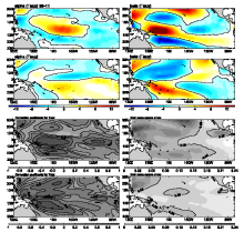
Spatial patterns of the coefficients of the regression relationships in 1999-2011 (Fig. 3) are quite different from those in the preceding sub-period: both zonal and meridional wind stress anomalies are mainly dominated by the SST over the Niño4 region. Due to the more westerly position of the Niño4 region compared to the Niño3 region, these patterns mean a westward shift of the wind patterns compared with those in the former sub-period. The correlation coefficients and RMSEs between the regressed wind stresses and the original wind stress data in this sub-period also indicate the regression relationships constructed are quite reasonable (Fig. 3). The satisfactory performance of the regression relationships between wind stress anomalies and Niño3 and Niño4 indices in both sub-periods not only indicates the strong coupling nature between atmosphere and ocean over the tropical Pacific, but also that the decadal changes of the interannual air-sea interactions can be quite effectively captured by this simple method.
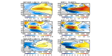
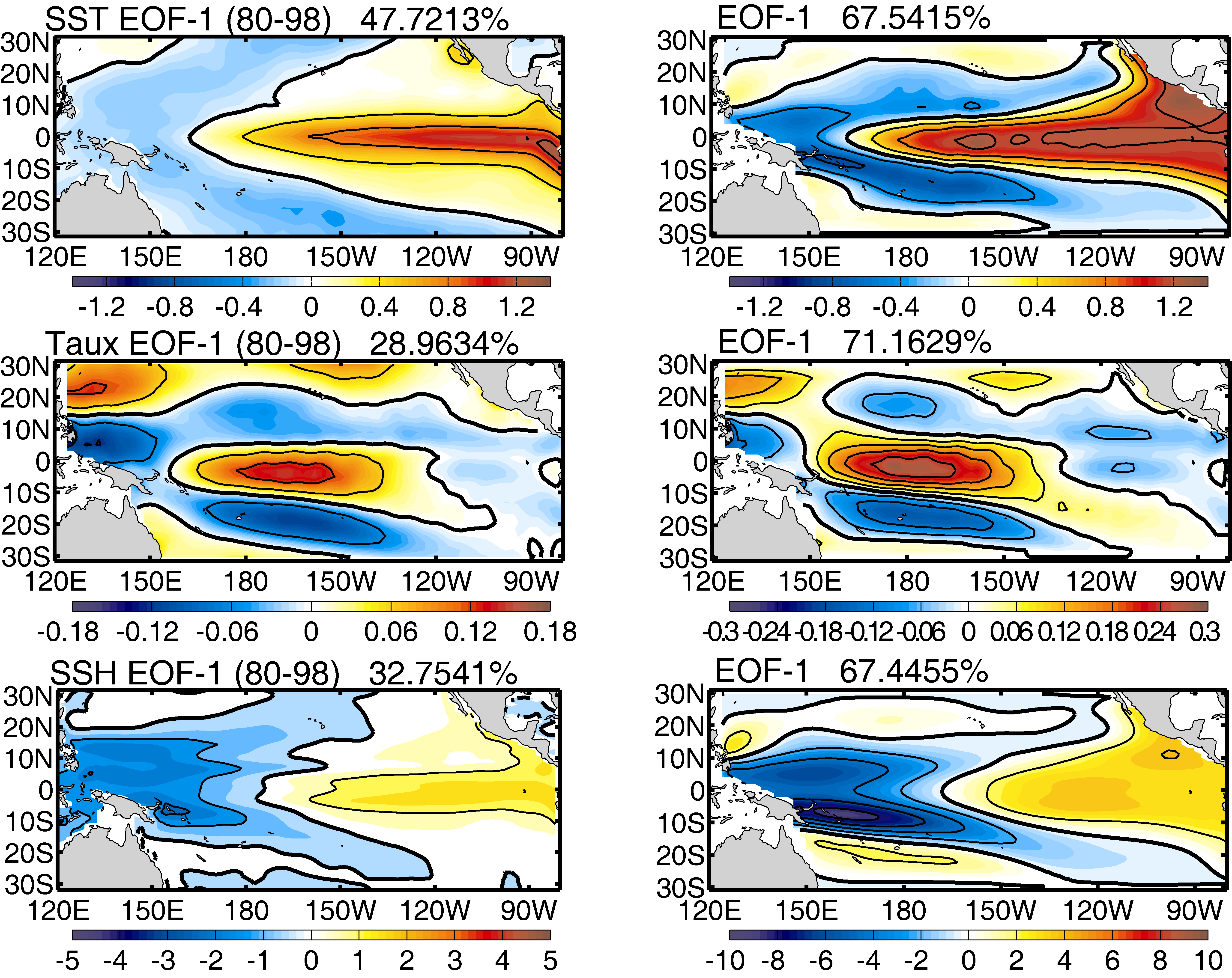
These regression relationships are also embedded in the GMODEL to test what predominant patterns will occur, and this experiment is named Exp2. For comparison, the leading EOF patterns of anomalous SST, zonal wind stress, and SSH based on the observed data in 1999-2011 are shown in the left-hand panels of Fig. 4, which manifest the CP El Niño patterns, different from those in the preceding sub-period: a major warming center is situated in the central Pacific while the lateral V-shape cooling pattern is located in the far west; the westerly wind stress anomalies are also in the central and western Pacific, but with a westward shift, and the easterlies in the eastern Pacific have a larger zonal stretch and amplitude; positive SSH anomalies also have a westward shift and are located in the central and eastern Pacific, while negative ones are limited in the west and with a narrow zonal stretch too. These corresponding changes are reflected in the changes of the regression relationships between the two sub-periods, as mentioned above. These EOF analyses also reflect the fact that CP El Niño is the predominant warming event in the most recent decade. The leading EOF patterns of the corresponding results of Exp2 are shown in the right-hand panels of Fig. 4, which also show a high level of similarity with the left-hand panels, albeit with the shortcomings mentioned in the analysis of Fig. 2 still in existence. This indicates that the dominant occurrence of CP El Niño in the most recent decade is also largely dominated by the interannual wind-temperature relationships during this time. In other words, which type of El Niño prevails depends mainly on the corresponding interannual wind-temperature relationships during the period.
 | Figure 1 Coefficients of the regression relationships between wind stress anomalies and Niño3 and Niño4 SST indices (top two rows) in 1980-98, divided by air density (1.3 Kg m-3) and drag coefficient (0.0015), and correlations and the RMSE (dyn cm-2) between the observed and regressed wind stresses (bottom two rows). |
 | Figure 2 Leading EOF modes of SST (°C, top panels), zonal wind stress (dyn cm-2, middle panels), and SSH (cm, bottom panels) of the observed data in 1980-98 (left column) and the results from Exp1 (right column). |
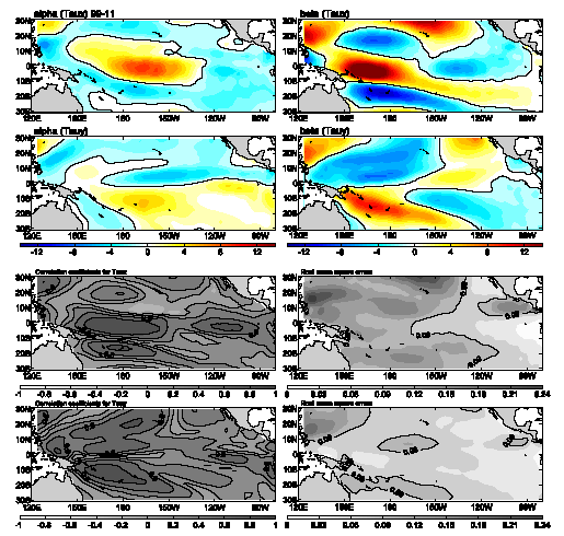 | Figure 3 Coefficients of the regression relationships between wind stress anomalies and Niño3 and Niño4 SST indices (top two rows) in 1999-2011, divided by air density (1.3 Kg m-3) and drag coefficient (0.0015), and correlations and the RMSE (dyn cm-2) between the observed and regressed wind stresses (bottom two rows). |
 | Figure 4 Leading EOF modes of SST (°C, top panels), zonal wind stress (dyn cm-2, middle panels), and SSH (cm, bottom panels) of the observed data in 1999-2011 (left column) and the results from Exp2 (right column). |
Due to the GMODEL being an anomalous model, it cannot depict exact mean state changes, but the EOF analyses of the anomalous fields can be used to illustrate what patterns are most likely to occur under the decadal changes of the interannual air-sea interactions. For this, the climate mean state over the tropical Pacific, the differences between the two experiments are first calculated by subtracting the results of Exp1 from those of Exp2, and then EOF analysis of each field is performed. The results are shown in the right-hand panels of Fig. 5. For comparison, background changes based on the observed data are also shown in the left-hand panels. It can be seen that the leading EOF patterns of the differences are quite similar to the mean state changes of the most recent decade, i.e., SST and SSH decreases in the eastern Pacific and increases in the west; and anomalous easterly winds occurring in the central and western Pacific and anomalous westerly winds in the east. This indicates that the La Niña-like mean state changes that occurred in the most recent decade, which in Xiang et al. (2012) are argued to have led to the predominance of CP El Niño, likely developed because of decadal changes in interannual air-sea interactions.
In this work, the regression relationships between anomalous wind stresses and Niño3 and Niño4 indices are constructed for 1980-98 and 1999-2011 to represent the interannual air-sea interactions over the tropical Pacific regions, and show reasonable performance (Figs. 1 and 3). These relationships are then embedded in a linear coupled model of the equatorial Pacific (GMODEL V3.0) to investigate how decadal changes of the relationships of interannual variabilities can influence the climate mean state. The results indicate that the respective predominance of EP and CP El Niño in the two sub-periods is mainly dominated by relationships between anomalous wind stresses and SST. Furthermore, changes of these relationships between the two sub-periods are likely to induce La Niña-like patterns, which are similar to the climatic changes that occurred in the most recent decade.
 | Figure 5 Mean state changes (1999-2011 minus 1980-98) of SST (°C, top panels), zonal wind stress (dyn cm-2, middle panels), and SSH (cm, bottom panels) based on the observed data (left column), and leading EOF modes of the differences between Exp1 and Exp2 (right column). |
Xiang et al. (2012) argued that such La Niña-like mean state changes prompt the generation of CP El Niño, while the results in this work emphasize that the interannual wind-temperature relationships can largely dominate the type of El Niño, and changes in the relationships can in turn modulate the mean state conditions. Very recently, England et al. (2014) also argued that no climate model can reproduce the La Niña-like background changes mentioned in this study, which they put down to the smaller- than-observed amplitude of modeled Pacific trade winds. In other words, this indicates that no climate model can capture the changes in interannual wind-temperature relationships either, and so what causes these changes is a very important question that should be explored in future studies.
Acknowledgments. This work was supported by the National Program for Support of Top-notch Young Professionals, the National Basic Research Program of China (Grant Nos. 2012CB955202 and 2012CB417404), 'Western Pacific Ocean System: Structure, Dyna-mics, and Consequences' of the Chinese Academy Sciences (WPOS; Grant No. XDA10010405), and the National Natural Science Foundation of China (Grant No. 41176014).
| 1 |
|
| 2 |
|
| 3 |
|
| 4 |
|
| 5 |
|
| 6 |
|
| 7 |
|
| 8 |
|
| 9 |
|
| 10 |
|
| 11 |
|
| 12 |
|
| 13 |
|
| 14 |
|
| 15 |
|