


Analysis of Nonstationary Wind Fluctuations Using the Hilbert-Huang Transform
[XU Jing-Jing1, 2 , HU Fei2, *  ]
]
]
|
|


Climatological patterns in wind fluctuations on time scales of 1-10 h are analyzed at a meteorological mast at the Yangmeishan wind farm, Yunnan Province, China, using a 2-yr time series of 10-min wind speed observations. For analyzing the spectral properties of nonstationary wind fluctuations in mountain terrain, the Hilbert-Huang transform (HHT) is applied to investigate climatological patterns between wind variability and several variables including time of year, time of day, wind direction, and pressure tendency. Compared with that for offshore sites, the wind variability at Yangmeishan wind farm has a more distinct diurnal cycle, but the seasonal discrepancies and the differences according to directions are not distinct, and the synoptic influences on wind variability are weaker. There is enhanced variability in spring and winter compared with summer and autumn. For flow from the main direction sector, the maximum wind variability is observed in spring. And the severe wind fluctuations are more common when the pressure tendency is rising.
Large fluctuations in wind speed on timescales of 1-10 h play an important role in energy and mass exchange between the surface and atmosphere, air pollution diffusion, and especially in the power management of large wind farms. For example, because of the high concentration of turbines within a small geographical area, fluctuations in wind speed can lead to severe power fluctuations for large offshore wind farms. For example, the power output from the 160-MW Horns Rev wind farm fluctuated up to 100 MW in a 15-20 min period according to a study by Akhmatov et al. (2007). Consequently, large-amplitude wind variability is quickly becoming a crucial problem for the wind energy industry ( Freedman et al., 2008).
Understanding wind variability on multiple timescales also has implications for both statistical and physical modeling, simulation and forecasting of wind speeds. The climatological trends of wind speed and other meteorological variables are of relevance to develop forecasting models, because they give clues with regard to the important explanatory factors that should be considered ( Vigueras-Rodriguez et al., 2010). For example, in a study by Sørensen et al. (2008), the stochastic properties of wind speed were used as an input for a model in simulating wind farm power fluctuations.
There are several arguments to suggest that wind speed time series must be nonstationary on multiple timescales ( Andreas et al., 2008; Post and Karner, 2008). Several authors have addressed the seasonal and diurnal patterns of wind variability, and its climatological patterns with regard to other variables ( Davey et al., 2010; Vincent et al., 2010, 2011). For analyzing the spectral properties of a nonstationary time series in which traditional global spectral analysis methods such as the Fourier transform do not work, an adaptive spectral analysis method called the Hilbert-Huang transform (HHT) has been adopted ( Huang et al., 1998) and successfully applied to many nonstationary meteorological and hydrological time series ( Rao and Hsu, 2008; Hsieh and Dai, 2012). In this paper, the HHT is used to study wind fluctuations at Yangmeishan wind farm in the southwest of China on temporal scales of 1-10 h, based on a 2-yr time series of 10-min wind speed observations. The aim of our work is to investigate climatological patterns between wind fluctuations and several potential explanatory variables including time of year, time of day, wind direction, and pressure tendency in mountain terrain compared with those of offshore sites.
The structure of the paper is as follows. In section 2, the observation site and the data are described. In section 3, a brief theoretical summary of the HHT and its specific use in this study is provided. The results are presented in section 4, and concluding remarks are given in section 5.
The analysis is based on measurements from a 70-m-high meteorological mast (25°06'N, 103°49'E; altitude: 2210 m). The mast is located close to the northwest of the Yangmeishan wind farm, Yunnan Province, China. There are 66 1.5-MW turbines in the wind farm, with the turbine height being 65 m. The surface conditions of the wind farm are typical of mountain terrain in Southwest China. The measurement mast is located to the northeast of Yangmeishan Mountain (Fig. 1). Therefore, at the Yang-meishan wind farm, wind from southwesterly directions approaches the wind farm from Yangmeishan Mountain.
The mast is equipped with cup anemometers at heights of 10, 65, and 70 m, wind vanes at heights of 10 and 65 m, and pressure and temperature sensors at heights of 8 m. In this study, a 2-yr time series (2010-11) of 10-min average wind speeds from the 65-m cup anemometer is used. For studying the relationship between wind variability and wind direction, measurements from the 65-m wind vane are used. Pressure measurements are also used to study the relation between wind variability and pressure tendency.
In this section, we first briefly summarize the theory of HHT, which was described in detail by Huang and Wu (2008). The HHT consists of three steps: empirical mode decomposition (EMD) of the time series into a set of intrinsic mode functions (IMFs); normalization of the IMFs and extraction of instantaneous amplitudes; and finally, extraction of instantaneous frequencies from the normalized IMFs using the Hilbert transform.
With the definition of an IMF ( Huang et al., 1998), the time series, U( t), can be decomposed through a sifting process. The EMD begins by extracting the fastest oscillations. Two cubic splines are defined: one passes through all the local maxima of the time series, and the other passes through all the local minima. The average of the two splines is considered the local mean of the data and is subtracted from the original time series. Therefore, the process is repeated until the remaining signal satisfies the conditions of being an IMF, i.e., that each maximum-min-imum pair is separated by a zero crossing. When the first IMF, x1( t), has been calculated, it is subtracted from the original signal, U( t), to obtain U1( t). The second IMF, x2( t), is then extracted from U1( t), and so on. When the time series has been decomposed into the IMFs xi( t), it may be written as
| , (1) |
where N is the number of IMFs into which the time series is decomposed, and
By modification to the Hilbert-Huang transform ( Huang and Wu, 2008), which proposes normalizing the IMFs so that they have constant amplitude of unity. This avoids the potential problem of the spectrum of an IMF overlapping the spectrum of its envelope. Normalization separates each IMF into an amplitude modulation part, Ai( t), and a frequency modulation part, Fi( t), so that
| (2) |
The normalized IMFs satisfy the special property that 400 500 600 700 800 900 1000 1100 1200 1300 1400 1500 1600 1700 1800 1900 2000 2100 2200 they each contain one unique frequency at each time, so that instantaneous frequencies can be calculated using the Hilbert transform. For each IMF, we can write
| , (3) |
where hi( t) is the Hilbert transform of xi( t), and PV denotes the principal value of the integral due to the singularity at
| (4) |
where Im means the imaginary part of the complex number.
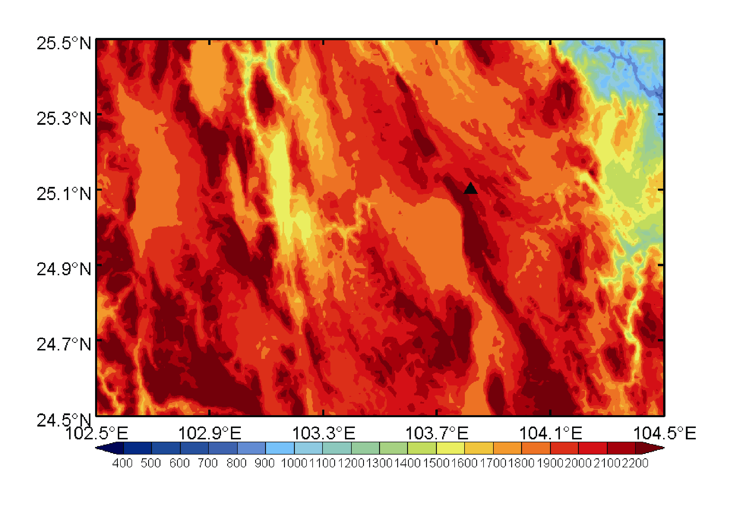 | Figure 1 Map of the northeast of Yunnan Province. The black solid triangle shows the location of the Yangmeishan wind farm. |
The Hilbert spectrum,
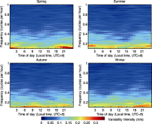
Wind variability may be relevant to time of year, diurnal cycle, synoptic cycle, and convective conditions. In this section, we first investigate the diurnal cycle and seasonal dependence of wind variability for timescales from 1 to 10 h. The 2-yr, two-dimensional Hilbert spectra are averaged into hourly time-of-day bins for each season. That is, 24 conditional spectra are created, one for each time of day (local time is used here for convenience), with each bin containing approximately 1095 observations. The averaged Hilbert spectra for the four seasons are shown in Fig. 2.
Because of the characteristics of the HHT, we focus on the low-frequency period in Fig. 2. That is, the frequencies between 0.1 cycles per hour and 0.33 cycles per hour. Figure 2 shows that the highest variability occurs in winter, and the plot shows enhanced variability in spring and winter compared with summer and autumn. However, compared with the offshore site ( Vincent et al., 2010), the wind variability at Yangmeishan wind farm has weaker seasonal discrepancies and a more distinct diurnal cycle. This may be caused by the different climatological and topographical conditions between land and offshore sites. So, for the diurnal cycle, there is a distinct high-amplitude period at night in spring, and a relatively high-amplitude period from 1800 LST to 2200 LST in winter, whereas a relatively low-amplitude period in the afternoon in summer.
The 2-yr time series of variability for periods of 1-3 h are also averaged into hourly bins, so the diurnal cycle in wind variability for high frequencies can be directly compared with the diurnal cycle in wind speed. Wind variability and wind speed as a function of time of day for the four seasons are shown in Fig. 3. From Fig. 3, we can see that the strongest wind speed is in winter, and the wind speed is also strong in spring compared with summer and autumn. This phenomenon differs from the wind speeds being strongest in autumn and winter in most monsoon areas. Moreover, the wind speed has an evident diurnal cycle in which, for each season, there is a peak between afternoon and night.
The wind variability also has a distinct diurnal cycle. However, the diurnal cycle in wind variability does not simply follow that of wind speed. There is considerable positive correlation between average wind speed and average variability except in autumn. Compared with the offshore site ( Vincent et al., 2010), the wind variability for high frequencies also has weaker seasonal discrepancies and a more distinct diurnal cycle. From Fig. 3, we can see that in spring, there is a late-afternoon maximum in wind speed, which is followed by a maximum in wind variability around 3-4 h later. The afternoon maximum in wind speed may be caused by the formation of a low-level jet ( Stull, 1988), and the maximum wind variability occurs when the low-level jet is decreasing in strength. A similar conclusion can be deduced in winter. In summer, a midday minimum in wind speed is observed and is followed by a minimum in wind variability around 1-2 h later. In autumn, two daily peaks in wind variability and one peak in wind speed are seen, which is different from the other three seasons.
Wind variability is expected to be dependent on wind direction due to the local surface conditions when the flow comes from particular directions, and to the preferred directions in certain synoptic conditions. The average Hilbert spectrum as a function of wind direction is created by classifying the spectra into 18 direction bins of width 20° for four seasons. The total bin sizes for each season for two years of data are shown in Fig. 4, where each bin contains approximately 1460 spectra. The main preferred direction range is between 200° and 240°, especially in spring and winter. The most frequent winds occur in the southwest sector, while the wind speeds are greatly suppressed for the northwest and northeast sector. The above phenomenon may be caused by the specific terrain of Yangmeishan Mountain.
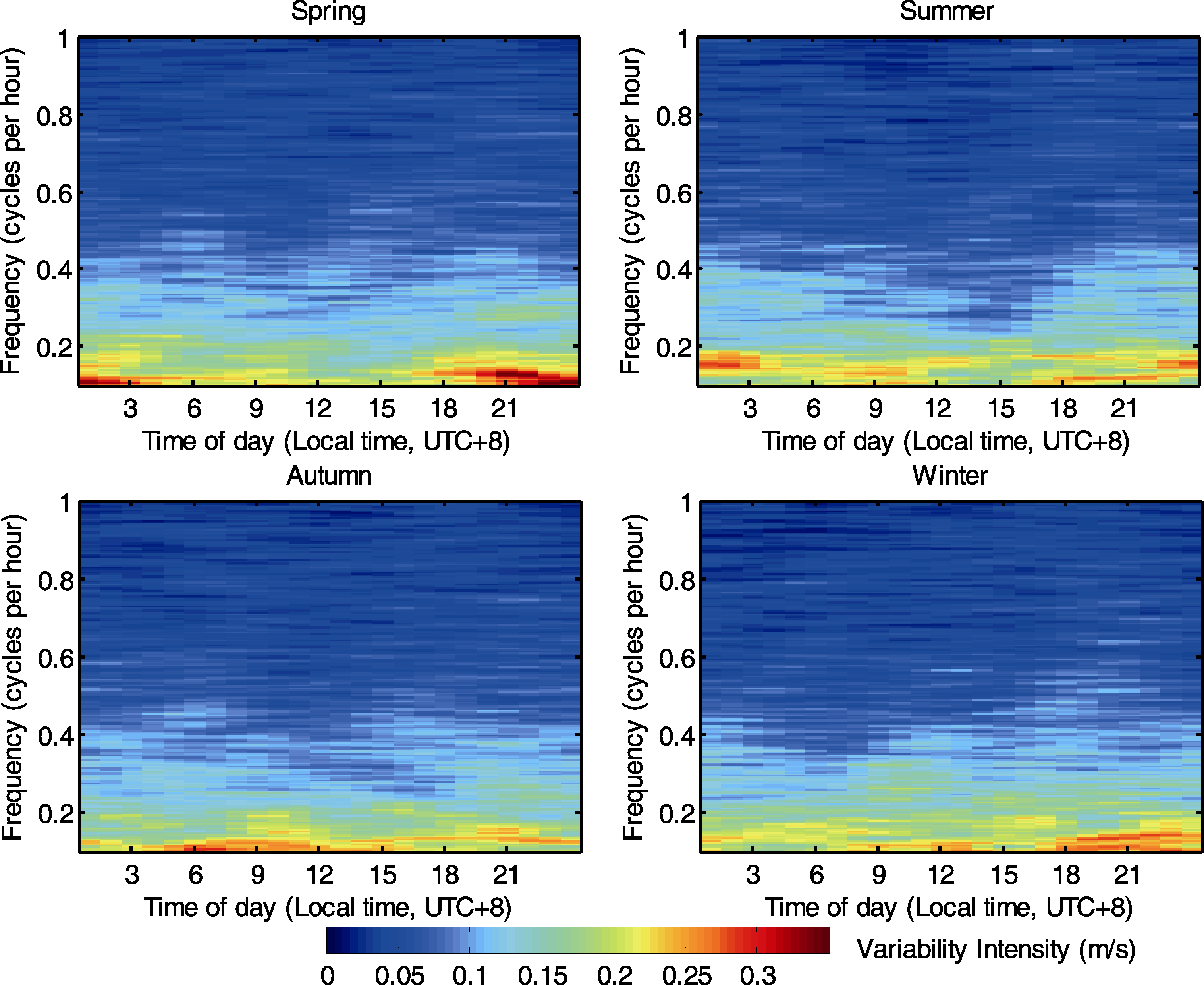 | Figure 2 Diurnal Hilbert spectrum averaged for the years 2010-11 for frequencies between 0.1 cycles per hour and 1 cycle per hour. |
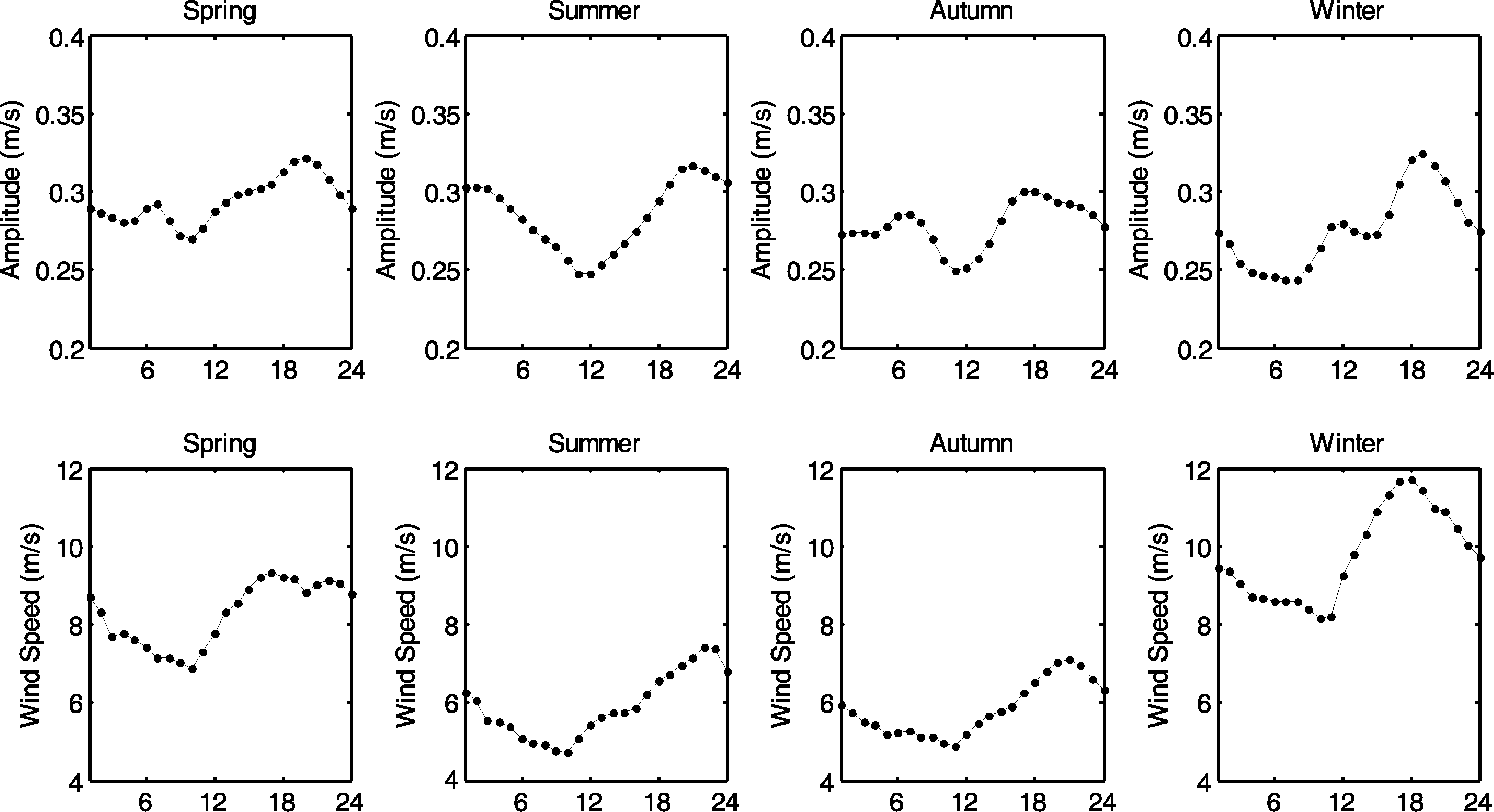 | Figure 3 Total amplitude of variability on scales of 1-3 h as a function of time of day, averaged for the years 2010-2011 (top). Wind speed as a function of time of day, averaged for the years 2010-2011 (bottom). The time of day is local standard time (LST). |
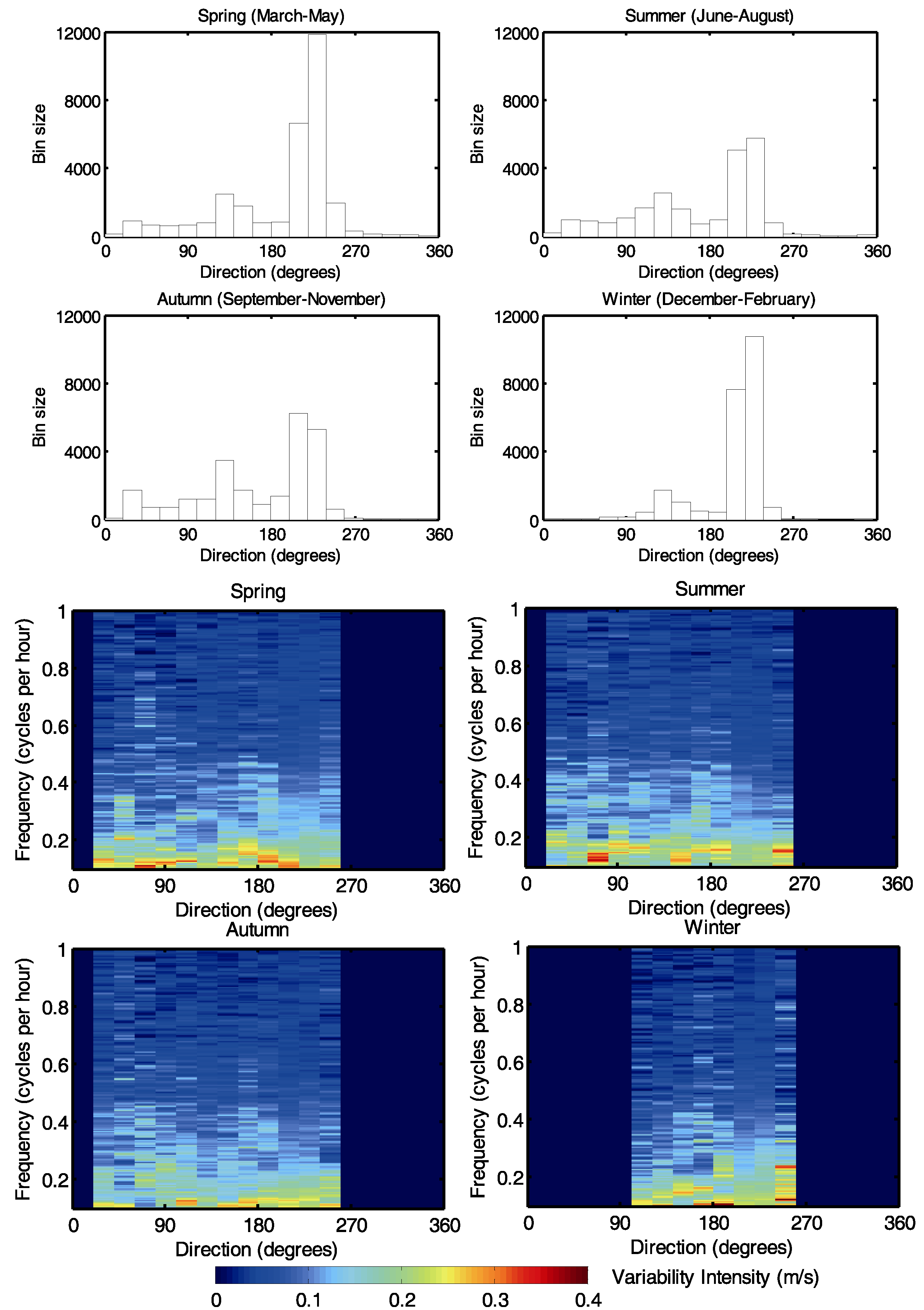 | Figure 4 Number of observations in each direction bin for four seasons for the years 2010-11 (top). Two-year averaged Hilbert spectrum according to wind directions (bottom). The bins that have spectrum numbers below 500 have been removed. |
The average Hilbert spectra as a function of wind direction and frequency for the four seasons are shown in Fig. 4. Because the directions are suppressed into several specific ranges, the bins that have spectrum numbers below 500 are removed, so according to other more representative bins, enough data are used in the analysis to ensure reasonability in the results. From Fig. 4, we can see that the differences according to directions are not distinct, and the seasonal discrepancies are also not obvious. This differs from more strongly preferred directions for more intense wind fluctuations in offshore sites caused by sea-land circulation ( Vincent et al., 2011). Moreover, some noticeable features are reflected. So, regarding the main direction range between 200° and 240°, the maximum variability is observed in spring. Wind variability in flow from the 180°-220° sector is exaggerated compared with other sectors in spring, and the maximum variability is found in a narrow range of directions of 60°-80° in summer. In autumn, variability is generally less than that in the other three seasons, while there is enhanced variability seen clearly in spring and summer for the low-frequency period. This analysis is highly site specific because of different synoptic patterns and surface conditions of various direction sectors. The reasons for the relationship between the wind variability and directions are difficult to describe from this analysis, and are interesting for further analysis by obtaining high-resolution topographical and land use data.
To test synoptic influences on wind variability simply, the variability spectrum conditional on the three-hourly pressure tendency is calculated. Positive values mean that the pressure is rising, i.e., the synoptic situation is post-frontal; negative values mean that the pressure is falling, and that the synoptic situation may be pre-frontal. The pressure tendency is divided into 13 bins, each of which has a width of 0.5 hPa per 3 h, so there are at least 2500 observations in each bin. The averaged spectrum for the low-frequency part (Fig. 5) shows a slightly stronger tendency for increased variability when the pressure is rising fast (in post-frontal conditions) than when the pressure is falling fast (in pre-frontal conditions). However, when the pressure tendency is close to zero, the wind variability is suppressed. The result that the greatest wind variability is experienced with the passage of a front is similar to the corresponding result in Vincent et al. (2011); however, the synoptic influences on wind variability in mountain terrain are weaker than those for offshore sites.
In this study, we apply the Hilbert-Huang transform to analyze nonstationary wind fluctuations in mountain terrain using wind observations from a meteorological mast at the Yangmeishan wind farm. The HHT is employed to obtain conditionally averaged spectra, and to investigate climatological patterns between wind fluctuations and several potential explanatory variables including time of year, time of day, wind direction, and pressure tendency in mountain terrain compared with offshore sites.
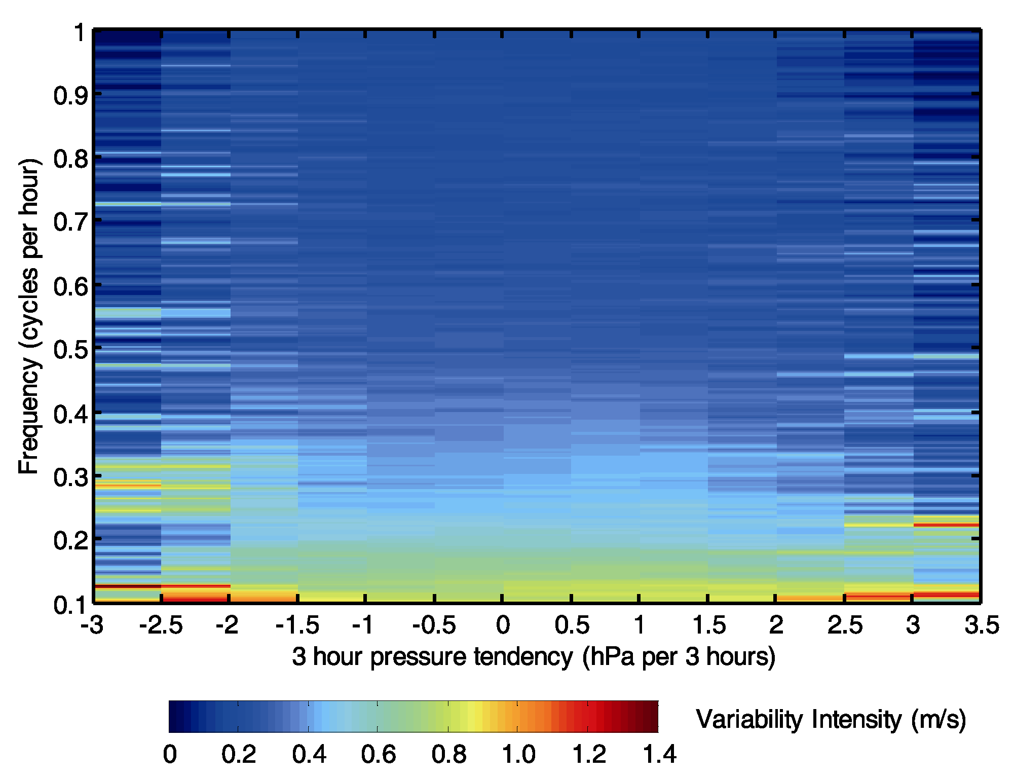 | Figure 5 Hilbert spectrum averaged for the years 2010-11 according to three-hourly pressure tendency. |
Due to the different synoptic patterns and surface conditions, the features of wind variability in mountain terrain differ from those for offshore sites considerably. The wind variability at Yangmeishan wind farm has a more distinct diurnal cycle, but the seasonal discrepancies and the differences according to directions are not obvious, and the synoptic influences on wind variability are weaker. Further, there are some other features for this specific site. There is enhanced variability in spring and winter compared with summer and autumn. And there is considerable positive correlation between wind speed and variability except in autumn. In spring and winter, there is a late-afternoon maximum in wind speed followed by a maximum in wind variability due to the formation of a low-level jet. In summer, a midday minimum in wind speed is observed and is followed by a minimum in wind variability. Furthermore, it is shown that for flow from the main direction sector, the maximum wind variability is observed in spring. The severe wind fluctuations are more common in post-frontal situations.
This study could be extended in the following aspects: the conditional spectra could be applied to other conditions of interest, such as atmospheric stability, or precipitation; and the methods could be applied to study the characteristics of higher frequency wind data such as turbulence. Furthermore, a newly developed method'the ensemble empirical mode decomposition (EEMD)'could be used to help the direct physical interpretation of individual IMFs.
Acknowledgments. This research was supported by the National Natural Science Foundation of China (Grant Nos. 91215302 and 41101045) and the 'One-Three-Five' Strategic Planning of the Institute of Atmospheric Physics, Chinese Academy of Sciences (Grant No. Y267014601).
| 1 |
|
| 2 |
|
| 3 |
|
| 4 |
|
| 5 |
|
| 6 |
|
| 7 |
|
| 8 |
|
| 9 |
|
| 10 |
|
| 11 |
|
| 12 |
|
| 13 |
|
| 14 |
|