This study used the coupled model of version 4 of the Community Atmosphere Model ( CAM4; Neale et al., 2013) and version 4 of the Community Land Model ( CLM4; Oleson et al., 2010; Lawrence et al., 2011). These are the atmosphere and land components of the Community Earth System Model (CESM), respectively. In CLM4, when the carbon-nitrogen model (CN) and the dynamic vegetation model ( CNDV; Castillo et al., 2012) are inactive, prescribed LAI data are needed as the boundary condition. LAI data have seasonal but no interannual variability. The model calculated daily LAI by interpolating monthly LAI between the closest two months. This may not accurately represent the mean state of land surface vegetation. Therefore, we used the interannual LAI data instead to characterize the status of land surface vegetation.

We used the Global LAnd Surface Satellite (GLASS) LAI dataset ( Liang et al., 2013) for 1982-2000. The spatial resolution of the GLASS LAI dataset is 0.05°, and the temporal resolution is eight days. The CESM simulation had a spatial resolution of 0.9° × 1.25°, and each grid cell was divided into 16 Plant Functional Types (PFTs) besides bare soil. To prepare the LAI data at CESM resolution, we applied the Moderate Resolution Imaging Spectroradiometer (MODIS) Land Cover Types dataset (MOD12C1) from the year 2000 (i.e., the data closest to the simulation period) at a resolution of 0.05°, and aggregate GLASS LAI dataset into each CESM land surface grid cell under the MODIS land cover type classification (Type 5, Class PFT). LAI values under each MODIS classification were assigned to corresponding CLM PFTs under each grid cell (Table 1). The fractional coverage of PFTs in each grid cell was also adjusted in order to preserve the grid- averaged LAI.

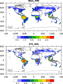
Figure 1 shows the spatial distributions of the annual mean LAI and its interannual variability evidenced by the standard deviation. The mean LAI was spatially heterogeneous. The highest values were found in tropical ecosystems, followed by temperate and boreal forests. Correspondingly, the same pattern occurred in its interannual variability. The standard deviation over the tropics exceeded 0.3, especially over the Amazon and Central Africa. On the global scale, the LAI was initially lower‘especially in 1988, 1992, and 1994‘and showed marginal increases more recently (Fig. 2).

Climatological LAI data were derived by averaging the new LAI data from 1985 to 2000. Both the climatological LAI data and the interannual LAI data were used in offline and online simulations.

Table 1

Table 1

Table 1 The relationships between Global LAnd Surface Satellite (GLASS)/Moderate Resolution Imaging Spectroradiometer (MODIS) and Community Land Model (CLM4) PFTs classifications. GLASS/MODIS CLM4 PFTs Evergreen broadleaf tree Deciduous broadleaf tree Evergreen needleleaf tree Deciduous needleleaf tree Shrub Grass Crop Tropical evergreen broadleaf tree Temperate evergreen broadleaf tree Tropical deciduous broadleaf tree Temperate deciduous broadleaf tree Boreal deciduous broadleaf tree Temperate evergreen needleleaf tree Boreal evergreen needleleaf tree Boreal deciduous needleleaf tree Temperate deciduous shrub Boreal deciduous shrub Evergreen shrub C4 grass C3 grass C3 arctic grass Crop

Table 1 The relationships between Global LAnd Surface Satellite (GLASS)/Moderate Resolution Imaging Spectroradiometer (MODIS) and Community Land Model (CLM4) PFTs classifications.

Figure 1

	Figure Option ViewDownloadNew Window
	Figure 1 (a) Annual mean LAI from 1985 to 2000 (m2 m-2); (b) Standard deviation of annual LAI.

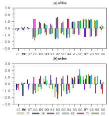
Figure 2 shows the standardized anomalies of global mean LAI, as well as the differences of offline and online simulations in ground temperature, evapotranspiration, and its three components: canopy transpiration, canopy

Figure 2

	Figure Option ViewDownloadNew Window
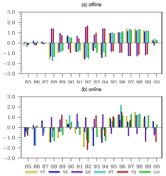	Figure 2 Standardized anomalies of LAI (green), as well as the differences between (a) offline simulations and (b) online simulations in evapotranspiration (ET, cyan) and its three components: transpiration (VT, yellow), canopy evaporation (VE, blue) and ground evaporation (GE, purple), as well as ground temperature (TG, red). All are averaged over the global land area.

evaporation, and ground evaporation. In the offline simulations, it was clear that, on the global scale, canopy transpiration, and evaporation were significantly positively correlated with LAI, whereas the correlation between ground evaporation and LAI was significantly negative. The correlation coefficients were 0.99, 0.99, and -1.0 respectively (Table 2). Furthermore, canopy transpiration and evaporation were more sensitive to changes of LAI, leading to a significantly positive correlation between total evapotranspiration and LAI. Consequently, the correlation between the ground temperature and LAI was significantly negative. This was because enhanced evapotranspiration not only favors cloud development, increasing reflection of additional solar radiation, but also consumes energy to convert water into water vapor, resulting in surface cooling.

The online simulations had substantially different correlations shown in Table 2. For example, for ground evaporation and evapotranspiration, the corresponding correlations decreased from -1.0 to -0.68 and from 0.97 to 0.56 respectively. On the other hand, for canopy transpiration and evaporation, the differences between online and offline simulations were small, indicating that these variables were more directly influenced by LAI.

Table 2

Table 2

Table 2 Regionally averaged correlations between the studied variables and leaf area index (LAI). VT* VE* GE* ET* TG* ABD* Offline Global 0.99 0.99 -1.0 0.97 -0.98 -0.56 30°S-30°N 0.98 0.99 -0.99 0.96 -1.0 0.62 45-75°N 0.97 0.98 -0.98 0.97 -0.74 -0.97 Online Global 0.96 0.88 -0.68 0.56 0.40 -0.42 30°S-30°N 0.97 0.89 -0.73 0.55 -0.70 0.15 45-75°N 0.77 0.81 -0.25 0.57 0.33 -0.67 *Variables VT, VE, GE, ET, TG, and ABD represent canopy transpiration, canopy evaporation, ground evaporation, evapotranspiration, ground temperature, and albedo respectively.

Table 2 Regionally averaged correlations between the studied variables and leaf area index (LAI).

The most significant change occurred in ground temperature, and the correlation coefficient changed from -0.98 in the offline simulations to 0.40 in the online simulations. To further investigate this phenomenon, sim-ilar analyses were conducted over low latitudes (30°S- 30°N) and middle to high latitudes (45-75°N). Besides evapotranspiration, albedo also plays an important role in influencing surface temperature. Their effects are opposite, i.e., warming through decreased albedo and cooling through intensified evapotranspiration. Table 2 shows that changes of LAI directly resulted in changes of surface albedo and evapotranspiration. In the online simulations, evapotranspiration and albedo were also influenced by changed climatic factors induced by LAI changes. These feedbacks, together with atmospheric variability, weakened the impact of evapotranspiration, resulting in red-uced correlation between evapotranspiration and LAI of 0.55 and 0.57, respectively, over both regions. They also changed the correlation between the albedo and LAI to 0.15 and -0.67. The warming effect of albedo over 45-75°N may have overcompensated for the cooling effect of evapotranspiration, resulting in a weak positive correlation between ground temperature and LAI. Thus, evapotranspiration and albedo tended to dominate at different latitudes. However, the above interactions may have been missed in the offline simulations due to the prescribed forcing inputs. The correlation between evapotranspiration and LAI over both regions was close to 1, leading to a stronger cooling effect that shaped the negative correlation between ground temperature and LAI. For this reason, coupled climate system models or earth system models may be more appropriate tools to fully investigate the influence of interannual vegetation variability.

In this subsection, we compare the effects of interannual vegetation variability on the interannual variabilities of ground temperature and evapotranspiration, as evidenced by the standard deviation (Fig. 3).

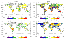
Generally, the spatial distribution of the differences between OFF-Int and OFF-Cli in interannual variability of evapotranspiration corresponded to that of LAI (Fig. 1). The main reason for this observation is that evapotranspiration was significantly positively correlated with LAI in offline simulations, as discussed above. Furthermore, the magnitude of the differences was small due to the lack of interaction between the land and the atmosphere. It should also be noted that, over tropical rainforest regions such as the Amazon, Central Africa, and South Asia, the interannual variability of evapotranspiration was less sensitive to the interannual variability of vegetation. The interannual variability of ground temperature in offline simulations also showed marginal differences, which did not exceed 0.1 K, except in the Amazon.

Figure 3

	Figure Option ViewDownloadNew Window
	Figure 3 The differences in the standard deviations of evapotranspiration (units: W m-2) between (a) OFF-Int and OFF-Cli and (b) ON-Int and ON-Cli, and of ground temperature (units: K) between (c) OFF-Int and OFF-Cli and (d) ON-Int and ON-Cli.

However, in the online simulations the overall fluctuation of differences in interannual variability of evapotran-spiration increased compared to those of the offline simulations. This difference spread over almost all land areas, i.e., it was not limited solely to vegetation growing regions. The atmospheric fluctuation and transportation played a significant role in this process. As for ground temperature, the difference also showed a large increase, and exceeded 0.1 K over large areas. The fifth assessment report (AR5) of the Intergovernmental Panel on Climate Change (IPCC) reported that the globally averaged combined land and ocean surface temperature data warmed by 0.85 ± 0.2°C from 1880 to 2012. Therefore, the influence of interannual vegetation variability should be considered in studies of uncertainty in climate change.