The REMO Ocean Data Assimilation System into HYCOM (RODAS_H): General Description and Preliminary Results
Cite this Article
Clemente Augusto Souza TANAJURA, Alex Novaes SANTANA, Davi MIGNAC, Leonardo Nascimento LIMA, Konstantin BELYAEV, XIE Ji-Ping. The REMO Ocean Data Assimilation System into HYCOM (RODAS_H): General Description and Preliminary Results. Atmospheric and Oceanic Science Letters, 2014, 7(5): 464-470 
Permissions
Copyright?2014, Editorial office of Atmospheric and Oceanic Science Letters
This is an Open Access article under the terms of CCAL.
The REMO Ocean Data Assimilation System into HYCOM (RODAS_H): General Description and Preliminary Results
Abstract
The first version of the Brazilian Oceanographic Modeling and Observation Network (REMO) ocean data assimilation system into the Hybrid Coordinate Ocean Model (HYCOM) (RODAS_H) has recently been constructed for research and operational purposes. The system is based on a multivariate Ensemble Optimal Interpolation (EnOI) scheme and considers the high frequency variability of the model error co-variance matrix. The EnOI can assimilate sea surface temperature (SST), satellite along-track and gridded sea level anomalies (SLA), and vertical profiles of temperature (
Keyword:
ocean data assimilation; ensemble optimal interpolation; observing system experiment; HYCOM; Atlantic Ocean
1 Introduction
Data assimilation methods are important scientific tools for meteorology and oceanography. They combine model outputs with observational data in a mathematically optimal or sub-optimal way, and produce the objective analysis with smaller errors than the model output. The analysis is used as the model initial condition for weather and climate forecasts ( Kalnay, 2003), and more recently for ocean weather forecasts under the framework of operational oceanography ( Dombrowsky et al., 2009). Data assimilation methods are also applied to produce long-term series of analysis for climate diagnostics studies ( Kalnay et al., 1996), and to support the development of observational systems. The latter is done by data assimilation experiments, called observing system experiments (OSEs), to investigate the relative importance of specific observations to the analysis and the forecasts ( Lea et al., 2013).
Data assimilation methods look for the minimum of a least-square deviation of the model state with respect to observations and to a model background (or prior) state when the observation and the background errors are known ( Evensen, 2003; Moore et al., 2011). Some of these met-hods are computationally quite expensive. For operational purposes, the choice of method is a crucial aspect.
In this paper, a recently constructed data assimilation system for the Hybrid Coordinate Ocean Model (HYCOM) is described and the first results of an OSE are shown. The system was developed by the Brazilian Oceanographic Modeling and Observation Network (in Portuguese, Rede de Modelagem e Observacão Oceanográfica (REMO)) to be a component of an operational ocean forecasting system for the Atlantic Ocean (www.rederemo.org) ( Tanajura and Belyaev, 2009; Lima et al., 2013). It was called the REMO Ocean Data Assimilation System for HYCOM (RODAS_H) and it was constructed under international collaboration with the HYCOM Consortium (www.hycom. org), the Global Ocean Data Assimilation Experiment (GODAE) Ocean View project ( Dombrowsky et al.,2009), and the Institute of Atmospheric Physics, Chinese Academy of Sciences (IAP/CAS). RODAS_H is based on the Ensemble Optimal Interpolation scheme (EnOI), following very closely the algorithms suggested in Xie and Zhu (2010), Yan et al. (2010), and Xie et al. (2011). The EnOI has proved to be efficient and adequate for operational purposes ( Oke et al., 2008). The next sections present details about the data, the model, the EnOI scheme, the OSE, results, and conclusions.
2 Data and methods
2.1 Data
The data employed in the assimilation were:(i) Daily sea surface temperature (SST) analyses from the Ocean Sea Surface Temperature and Sea Ice Analysis (OSTIA) with a (1/20)° resolution (ftp://data.ncof.co.uk/ ostia_ reanalysis/);(ii) 6988 vertical profiles of temperature ( T) and salinity ( S) from Argo (ftp://ftp.ifremer.fr/ifremer/argo/geo/atlantic_ ocean/); and (iii) Along-track sea level anomaly (SLA) data from the satellites Jason-1, Jason-2, and Envisat from Archiving, Validation and Interpretation of Oceanographic Satellites data (AVISO) (ftp://ftp.myocean.sltac.cls.fr/Core/).
The experiments were evaluated with these data, with SST analysis ( Reynolds et al., 2007) with a (1/4)° resolution (ftp://eclipse.ncdc.noaa.gov/pub/OI-daily-v2/NetCDF/), AVISO SLA gridded data with an absolute dynamical topography with a (1/3)° resolution (https://www.aviso. oceanobs.com), and Ocean Surface Current analyses (OSCAR) with a (1/3)° resolution (http://www.oscar.noaa.gov).
2.2 The ocean model
HYCOM is a generalized vertical coordinate model, which can assume isopycnal, terrain-following, or constant fixed depth ( z) coordinates. The coordinate is adjusted dynamically to the best option according to the ocean characteristics in each region around a prescribed potential density reference ( Bleck, 2002).
The model was configured with a spatial resolution of 0.25° and 21 vertical layers, of which 18 were hybrid and 3 were z-coordinate. The model domain covered almost all the Atlantic Ocean from 78°S to 50°N and from 100°W to 20°E, excluding the Pacific Ocean and the Mediterranean Sea. On the lateral boundaries, relaxation towards temperature and salinity climatology was applied, and constant barotropic volume fluxes were imposed ( Lima et al., 2013).
After a 40-year spin-up with climatological forcing, the model was forced by the National Centers for Environmental Prediction/National Center for Atmospheric Research (NCEP/NCAR) atmospheric reanalysis from 1 January 1993 to 31 December 2009 ( Kalnay et al., 1996) (ftp://ftp.cdc.noaa.gov/Datasets/ncep.reanalysis/surface_gauss/). The last 12 years of this model run were used to create the ensemble statistics for the EnOI scheme.
2.3 The data assimilation scheme
The analysis Xa according to EnOI is given by the formula ( Evensen, 2003)
| (1) |
where
| (2) |
where 
The 132 ensemble members used to calculate B were selected from the model free run for each assimilation day, considering the intra-seasonal variability and the high frequency model dynamics, as in Xie and Zhu (2010), Yan et al. (2010) and Xie et al. (2011). For instance, to perform assimilation on 15 March 2010, 11 members centered on 15 March of each year from 1998 to 2009 were taken with eight days between each member.
The diagonal matrix R in Eq. (2) depends on the observation type, and includes information about the instrumentation error (IE) and the representativeness error (RE). For SST and SLA data, the IEs were assumed to be 0.25°C and 0.04 m, respectively, following Oke et al. (2008) and Xie et al. (2011). The REs for SST and SLA were calculated according to Oke and Sakov (2008), using the super-observation approach. They were estimated from the standard deviation of the difference between the original data and a weighted average considering the distance between the original datum and the analysis point.
To assimilate along-track SLA data, the model SLA had to be extracted by first subtracting the model SSH from a SSH mean produced by the model free run from 1993 to 1999. However, the mean of the SLA data and the mean of the model SLA did not coincide. An offset of about 25 cm was observed. This was mainly due to the use of different reference surfaces to calculate the observed and the modeled SLAs. Therefore, an adjustment in the innovation was made. First, the average of the model SLA and the average of the AVISO SLA were calculated from 2000 to 2009. The offset was calculated by subtracting the AVISO average from the model average. Then, the model SLA was adjusted by subtracting the offset from the model SLA. The innovation was calculated with the adjusted model SLA, so that the meso-scale structure was highlighted.
For the Argo T-S data, the strategy by Xie and Zhu (2010) was employed. The first step was to create a pseudo-observation of the vertical profile of the model layer thickness (DPobs) for each Argo T-S profile based on the Argo data and on the model isopycnic coordinates. Then, DPobs was assimilated to create an analysis for (DP, U, V) in all the model layers. The next step was to assimilate T and S in the mixed layer, and S in the isopycnic layers, since previous works showed that most of the correction of the T profiles was done when DPobs was assimilated, and that assimilating S was the only effective way to constrain it ( Oke and Schiller, 2007; Xie and Zhu, 2010).
The horizontal radius of influence for SST, SLA, and the Argo data was set to 150 km and the localization operator was set to null co-variances for points separated by more than 300 km.
2.4 The observing sensitivity experiment
Five integrations forced with the NCEP/NCAR reanalysis were performed from 1 January to 30 June 2010. The first was a control run without assimilation. The other four assimilated different observations every three days: (i) only along-track SLA data (A_SLA); (ii) only SST analyses (A_SST); (iii) only vertical profiles T and S from Argo (A_Argo); and (iv) all data employed in the previous runs (A_All). When Argo data was assimilated, a three-day observational window was applied. For the other data, only a one-day observational window was considered.
The full capability of RODAS_H was realized in the A_All run according to the algorithm:(i) Assimilate the OSTIA daily SST data to modify (DP, U, V, S, Ubar, Vbar, Pbar) in the model column.
(ii) Integrate the model for 6 h and use the resulting state as background. Produce DPobs for each available Argo T-S profile, assimilate DPobs to modify (DP, U, V), and then assimilate T-S in the mixed layer and S in the isopycnic layers in a univariate way.
(iii) Integrate the model for 6 h and use the resulting model state as background. Assimilate along-track SLA to modify (DP, U, V, S, Ubar, Vbar, Pbar) in the model column.
(iv) Integrate the model for 60 h and perform a new assimilation cycle.
3 Results and discussion
Data assimilation was realized every three days in the four assimilation runs. On the assimilation day, the OSE results were assessed by comparing the prior state (before assimilation) of each run with daily SST analyses ( Reynolds et al., 2007), Argo T-S data from 6988 profilers, and gridded SLA data from AVISO. These data can be considered as independent, since they were not used by RODAS_H at the assessment time. The prior state of each run was evaluated daily from 1 January to 30 June 2010, and it is analogous to the evaluation of a 24-h forecast.
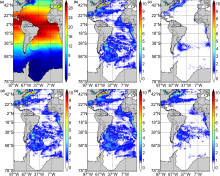
Comparison of the control run SST with Reynolds SST analysis showed that the largest differences were attained in the Gulf Stream (GS) region, in coastal areas in the southwest South Atlantic around 38°S and in the east South Atlantic around 18°S (Fig. 1). The maximum root mean square deviation (RMSD) of the control run were almost 10°C in the GS region, since this feature was displaced to the north of its observed position. In the majority of the model domain, the RMSD was below 2°C. The control run was warmer than the observations, particularly in the areas of large RMSD. When SST was assimilated, the RMSD was substantially reduced. The A_SST run attained maximum deviation between 3°C and 4°C in the GS region, and overall the RMSD was below 1°C. The A_Argo run reduced the RMSD of the control run mainly in the North Atlantic, where most of the Argo profilers were located. The A_SLA run did not produce any noticeable impact on SST. The A_All run was almost as effective as the A_SST run, since it substantially reduced the RMSD produced by the control run, but in some regions, such as the subtropical North and South Atlantic, the RMSD were between the ones attained by the control and the A_SST runs.
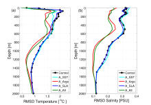
The maximum RMSD of T and S of the control run with respect to Argo data were produced in the top 200 m (Fig. 2). This is associated with the difficulties that models have representing the thermocline and pycnocline regions of sharp vertical gradients ( Oke and Schiller, 2007; Xie and Zhu, 2010). When Argo data were assimilated in the A_Argo and in A_All runs, the vertical structure of T and S of the prior state were very much improved. The maximum RMSD of T and S in the top 200 m were reduced from about 2.2°C to 1.6°C and from 0.35 psu to 0.2 psu, respectively. Assimilation of the SST reduced the control run RMSD of T in the top 400 m, but it had no impact in Tbelow 400 m or in S in the whole column. Actually, the RMSD of S increased a little at the surface with the A_SST run. The assimilation of SLA had no impact on either T or S.
These results highlight the importance of the Argo data to constrain the model. Only when these data were assimilated were the RMSD of T and Sof the prior state reduced from the surface down to about 1800 m. Also, the assimilation of S was particularly effective by reducing the RMSD of the control run by about 30% in the top 800 m and by 50% from 800 m to 1400 m. Between 0 and 300 m, A_Argo produced a smaller RMSD of T than A_All.
 | Figure 1 (a) Reynolds SST mean (°C) from 1 January to 30 June 2010 and root mean square deviation of SST with respect to Reynolds daily analyses according to (b) control run, (c) A_SST run, (d) A_Argo run, (e) A_SLA run, and (f) A_All run. |
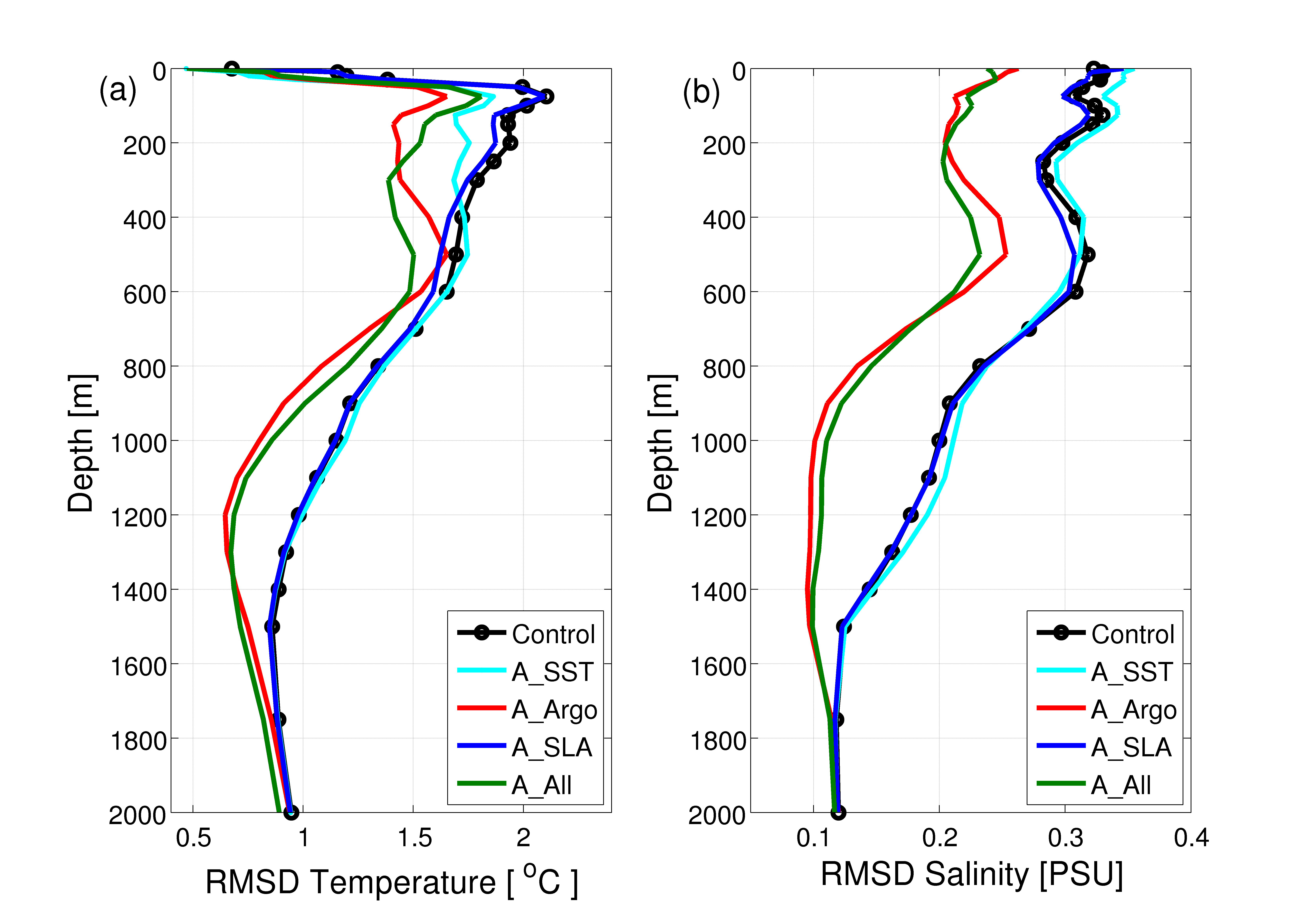 | Figure 2 Vertical profiles of the root mean square deviation for (a) temperature (°C) and (b) salinity (psu) against 6988 Argo profilers in the model domain (78°S-50°N, 100°W-20°E) from 1 January to 30 June 2010 according to the control run (black with circles), the A_SST run (light blue), A_Argo run (red), A_SLA run (dark blue), and the A_All run (green). |
However, between 300 m and 600 m, the opposite happened. This indicates a negative (positive) influence of the SST and SLA data in the subsurface structure of T in the A_All run in the layer between 0 and 300 m (300 and 600 m), and shows how important accurate ensemble co-variances of the model free run are for the EnOI to produce a good analysis.
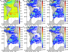
To assess the SLA RMSD, the SLA offset between model and observation was subtracted from the model SLA in all OSE runs. Nevertheless, the control run SLA showed large discrepancies with respect to the data. It was about 0.40 m in regions of strong meso-scale activity in the subtropics and mid-latitudes in both the North and South Atlantic, particularly in the GS and its extension towards Europe, in the Brazil-Malvinas Confluence and in the Benguela Current region (Fig. 3). The A_SST, A_Argo, and A_All runs could not reduce the SLA RMSD of the control run. They actually increased the RMSD in certain regions by 0.1 m, and this is discussed below. However, the A_SLA run produced a substantial reduction of RMSD with respect to the control run, including the areas with strong meso-scale activity.
Part of the RMSD increase produced by the A_SST, A_Argo, and A_All runs is associated with a problem in the metrics of assessing the impact of the assimilation on SLA and also with the calculation of the innovation. The same offset was used for all model runs, but it was clear that when the assimilation of SST and Argo data were realized, the model mean SSH changed, particularly with the Argo data. At the beginning of the integration, the model SSH averaged over the model domain north of 60°S was about 0.1 m (not shown). This value remained approximately the same along the A_SST and A_SLA runs. However, the SSH was reduced to 0.05 m and 0.075 m at the end of the A_Argo and A_All runs, respectively. The model free and control runs were in general warmer than the observation, so that when Argo data was assimilated, it increased the mean density in the water column and reduced the averaged model SSH. Therefore, inaccuracies were introduced to calculate the innovation and the SLA RMSD in the A_Argo and A_All runs when the offset based on the free run was employed. A different strategy that considered the SLA offset per satellite track was used in Tanajura et al. (2013). This approach will be explored in future experiments.
The surface currents were also objectively evaluated. The RMSD of the control run U and V with respect to OSCAR attained the largest values in the western subtropical and mid-latitudinal North Atlantic, about 0.9 m s-1 (figure not shown). This was associated with the misplaced GS. In the major part of the domain, the RMSD of U and V were between 0 and 0.1 m s-1. The A_SLA and A_SST runs did not substantially alter this picture, despite some reduction of the deviations in the North and South Atlantic subtropical regions. The A_Argo and A_All runs produced an increase of the deviations. This is mostly because cyclonic and anti-cyclonic circulations developed around the majority of the assimilated Argo profiles, consistent with the large local modifications of the model layer thicknesses and geostrophy ( Xie and Zhu, 2010).
To summarize the results of the OSE, the area-averaged RMSDs of SST and SLA from Fig. 1 and Fig. 3, and the vertical mean of the RSMD profiles of T and S from Fig. 2 are presented in Table 1. Table 1 also contains the RMSD of U and V with respect to OSCAR and the correlation of SLA with the AVISO data. The calculations were performed over the whole model domain, except for the SLA RMSD and correlation that excluded the region south of 60°S. As mentioned above, the smallest RMSDs of the prior state were not attained by the A_All run when compared to each assimilation run specifically. The smallest RMSD of SST, T and S, and SLA were attained by the A_SST, A_Argo, and A_SLA runs, respectively. They reduced the RMSD of the SST by 46% (from 1.51°C to 0.81°C), the RMSD of T by 21% (from 1.42°C to 1.12°C), the RMSD of S by 31% (from 0.26 psu to 0.18 psu), and the RMSD of SLA by 26% (from 0.078 m to 0.058 m). The correlation of SLA by the A_SLA run increased by 112% with respect to the control run (from 22.2% to 47.1%). The RMSDs of the control run surface U and V were 0.108 and 0.084 m s-1, respectively. These values increased by up to 12% in the assimilation runs, except for U in the A_SLA run. This increase reflects inaccuracies in the ensemble co-variances and in the background. A more complete investigation on the impact of the assimilation in the circulation will be done in future work.
 | Figure 3 (a) AVISO SLA mean (m) from 1 January to 30 June 2010 and root mean square deviation of SLA with respect to AVISO daily data according to (b) control run, (c) A_SST run, (d) A_Argo run, (e) A_SLA run, and (f) A_All run. |
Because of the relatively small impact on the model variables that were not assimilated, the A_All run produced a good performance when all assimilated variables were considered together. It consistently reduced the RMSD of SST, T, and S by 39%, 18%, and 30%, respectively, and increased the SLA correlation by 81%. In contrast to the large SLA RMSD, the A_All run improved the SLA correlation and the high frequency meso-scale variability.
4 Conclusions
The first results of RODAS_H showed that the system could assimilate SST, Argo T-S data, and along-track SLA from Jason-1, Jason-2, and Envisat, and improve the model state towards these observations. When all variables were assimilated in the same run, a good overall result was obtained, with substantial reductions of deviations with respect to observations. When SST, Argo T-S, and SLA data were assimilated separately, the system produced the best correction with respect to the specific variable that was assimilated, but had a small or negligible impact on the other variables. Among the reasons for this lack of sensitivity is the relatively short period of the OSE (only six months), and the low co-variance values produced by the ensemble members retrieved from the free run. Also, the parameter,
Assimilation of Argo T-S data was very effective in constraining these variables, particularly S. This shows the importance of the Argo data to correct the model thermohaline structure. Also, assimilation of Argo T-S data imposed a change in the model mean SSH and this introduced errors in the calculation of the innovation of SLA and in the accuracy of the analysis. However, the conflicts between the assimilation of Argo data and SLA, and the difficulty of the EnOI to objectively improve the circulation can be attributed to inaccurate co-variances produced by the model ensemble members. If the model free run and background state had some features of the large-scale circulation and thermohaline structure closer to climatology or observations, the assimilation would not have imposed for instance large changes in the model layer thicknesses and SSH. The A_All run would probably have led to smaller RMSDs than all the other assimilation runs. A better set of ensemble members will be pursued before RODAS_H is moved to operational mode in the REMO forecasting system.
| Table 1 Root mean square deviation (RMSD) of the prior state with respect to Reynolds SST analyses, 6988 Argo T and S profiles, AVISO SLA data, and OSCAR surface zonal ( U) and meridional ( V) velocities for each run from 1 January to 30 June 2010; and correlation coefficient (Corr) of SLA for each run with respect to AVISO data. The calculations were performed over the whole model domain (78°S-50°N, 100°W-20°E), except for the SLA RMSD and correlation that excluded the region south of 60°S. |
Acknowledgments. This work was financially supported by the Brazilian State oil company Petróleo Brasileiro S. A. (Petrobras) and Agência Nacional de Petróleo (ANP), Gás Natural e Biocombustíveis, Brazil, via the Oceanographic Modeling and Observation Network (REMO). The first author acknowledges support of the Coordenação de Aperfeiçoamento de Pessoal de Nível Superior (CAPES), Ministry of Education of Brazil (Proc. BEX 3957/13-6).
Reference
| 1 |
|
| 2 |
|
| 3 |
|
| 4 |
|
| 5 |
|
| 6 |
|
| 7 |
|
| 8 |
|
| 9 |
|
| 10 |
|
| 11 |
|
| 12 |
|
| 13 |
|
| 14 |
|
| 15 |
|
| 16 |
|
| 17 |
|