
Model-Simulated Atmospheric Carbon Dioxide: Comparisons with Satellite Retrievals and Ground-Based Observations
[WANG Jiang-Nan1, 2 , TIAN Xiang-Jun1, *  , FU Yu
3 ]
, FU Yu|
|


Atmospheric CO2 concentrations from January 2010 to December 2010 were simulated using the GEOS-Chem (Goddard Earth Observing System-Chemistry) model and the results were compared to satellite Gases Observing Satellite (GOSAT) and ground-based the Total Carbon Column Observing Network (TCCON) data. It was found that CO2 concentrations based on GOSAT satellite retrievals were generally higher than those simulated by GEOS-Chem. The differences over the land area in January and April ranged from 1 to 2 ppm, and there were major differences in June and August. At high latitudes in the Northern Hemisphere in June, as well as south of the Sahara, the difference was greater than 5 ppm. In the high latitudes of the Northern Hemisphere the model results were higher than the GOSAT retrievals, while in South America the satellite data were higher. The trend of the difference in the high latitudes of the Northern Hemisphere and the Saharan region in August was opposite to June. Maximum correlation coefficients were found in April, reaching 0.72, but were smaller in June and August. In January, the correlation coefficient was only 0.36. The comparisons between GEOS-Chem data and TCCON observations showed better results than the comparison between GEOS and GOSAT. The correlation coefficients ranged between 0.42 (Darwin) and 0.92 (Izana). Analysis of the results indicated that the inconsistency between satellite observations and model simulations depended on inversion errors caused by data inaccuracies of the model simulation's inputs, as well as the mismatch of satellite retrieval model input parameters.
In order to control global warming caused by rising atmospheric CO2 concentrations, the United Nations is calling for countries to implement relevant measures to reduce and control anthropogenic emissions (the Intergovernmental Panel on Climate Change (IPCC), 2007). Therefore, data on changes in atmospheric CO2 concentrations are an important basis for monitoring and evaluating reductions in CO2, and thus improving and developing emissions reduction policies, understanding the global carbon cycle, and revealing carbon sources and sinks.
Satellite remote sensing is fast becoming one of the most important means to quantitatively explore the temporal variation of atmospheric CO2, including the monitoring of both global- and regional-scale CO2 increases ( Reuter et al., 2011). Compared with ground observations, remote sensing can comprehensively cover most areas of the world. Examples of current orbiting satellites, or instruments onboard satellites, involved in observing atmospheric CO2 include the Atmospheric Infrared Sounder (AIRS), the Infrared Atmospheric Sounding Interferometer (IASI), and the Greenhouse Gases Observing Satellite (GOSAT).
For the orbiting satellites, the standard deviation of the most recent set of atmospheric CO2 concentration data released by the latest GOSAT, launched in 2009, is approximately 2 ppm-a figure verified by both ground and airborne observations ( Yokota et al., 2009). However, because ground-based observation stations are few in number and generally located far away from artificial emissions regions, station-based verification is insufficient to evaluate the accuracy of GOSAT observations. Therefore, we need additional methods to evaluate the accuracy of GOSAT data and reveal the spatiotemporal characteristics of atmospheric CO2 concentrations at the global and regional scales.
One such method, which has become hugely important for scientists working in this field of research ( Bey et al., 2001), is numerical modeling. Under this approach, atmospheric transport models such as GEOS-Chem (Goddard Earth Observing System-Chemistry) use meteorological data, anthropogenic emissions data, and data on carbon sources/sinks as inputs to simulate continuous spatiotemporal features of the global atmospheric CO2 concentration, enabling both qualitative and quantitative analyses of its variability and global delivery process.
While modeling can simulate a spatial and temporal continuum of the global atmospheric CO2 concentration, satellite remote sensing can objectively obtain information on global and regional atmospheric CO2 concentration changes using real-time observations. Therefore, model simulations and satellite observations provide us with atmospheric CO2 concentration data in two very different ways, but the differences between the two in terms of the features of global and regional atmospheric CO2 concentrations that they yield have yet to be comprehensively analyzed and evaluated. Accordingly, in the present reported study, we focused on comparing the global CO2 simulated by a 3D global chemical transport model (GEOS-Chem) with GOSAT retrievals from January 2010 to December 2010. To evaluate the model's performance, we used ground-based CO2 measurements from 14 stations, which enabled us to remove the model bias and better estimate the bias in the GOSAT CO2 observations. It is hoped that this work can help with preparations for a global CO2 data assimilation system.
The remainder of the paper is structured as follows. In section 2 we describe the retrieval of column-average dry-air mole fraction of CO2 ( XCO2) from GOSAT, as well as the observations from the Total Carbon Column Observing Network (TCCON). We also describe the GEOS- Chem model and the method used to convert the atmospheric CO2 concentration data to XCO2 (GEOS- XCO2). In section 3 we compare the GEOS- XCO2 results with GOSAT retrievals and TCCON data. And finally, the conclusions of the study are summarized in section 4.
GOSAT was the first satellite to measure atmospheric CO2 and methane (CH4). It carries two sensors: a Fourier Transform Spectrometer (FTS) and a Cloud and Aerosol Imager (CAI). Validation based on TCCON data has shown that GOSAT- XCO2 values are on average 0.3% (1.2 ppm) lower than TCCON observed XCO2 values, and the stan-dard deviation is approximately 2 ppm ( NIES GOSAT Project, 2010). The dataset used in the present paper is GOSAT-ACOS (Atmospheric CO2 Observations from Space)-v2.9.
The TCCON is an observation network of ground- based stations that use FTS instruments to gather information on CO2, CH4, and H2O. The solar spectrum is recorded in the near-infrared spectral region. From these spectra, the TCCON can provide accurate and precise column-averaged abundances of CO2 and CH4. TCCON observations have become a major source of information for validating and calibrating atmospheric CO2 concentration satellite retrieval data ( Wunch et al., 2011). The data can be downloaded fromhttp://tccon.ipac.caltech.edu/.
We collected XCO2 retrievals from January 2010 to December 2010 over 14 TCCON sites: Białystok (Poland); Bremen (Germany); Darwin (Australia); Eureka (Canada); Garmisch (Germany); Izana, Tenerife (Spain); Karlsruhe (Germany); Lamont, Oklahoma (USA); Lauder (New Zealand); Ny-Ålesund, Spitsbergen (Norway); Orléans (France); Park Falls, Wisconsin (USA); Sodankylä (Finland); Wollongong (Australia).
We simulated CO2 concentrations using GEOS-Chem (v9-01-03), the assimilated meteorological observations from GEOS of the National Aeronautics and Space Administration (NASA) Data Assimilation Office (DAO). The version of the model we used is driven by the GEOS-5 meteorology field with a horizontal resolution of 2° latitude by 2.5° longitude and 47 vertical layers.
The emissions data of the model include biogenic emissions, biomass emissions, and two other kinds of emissions data: Lightning Imaging Sensor and Optical Transient Detector (OTD-LIS) local redistribution, and Moderate-resolution Imaging Spectroradiometer (MODIS) derived leaf area index (LAI) ( Barkley, 2010). The biogenic emissions data are mainly from Model of Emissions of Gases and Aerosols from Nature (MEGAN) ( Guenther et al., 2006) and parameterized canopy environment emission activity (PCEEA) biological volatile organic compounds (BVOC) model data along with MEGAN MONO (monoterpenes) bio emissions. The biomass emissions data mainly include monthly Global Fire Emissions Database version 3 (GFED3) emissions ( van der Werf et al., 2010) and daily GFED3 emissions ( Mu et al., 2011).
Simulated data such as these can help us improve our understanding of the spatiotemporal distribution of global CO2 concentrations, as well as the carbon cycle. This approach has already been widely used by many researchers and research institutions worldwide to investigate global atmospheric CO2 concentrations, fluxes of carbon, and related aspects ( Baker et al., 2006). In the present study, we simulated the global CO2 concentration in the year of 2010 with 47 vertical levels and a horizontal grid resolution of 2° latitude by 2.5° longitude.
We converted the atmospheric CO2 concentration data in the model's 47 vertical levels to XCO2 in order to make the comparisons with the satellite data. The simulated data were weighted and converted into column-averaged concentration data using the averaging kernel function, thereby obtaining daily XCO2 data for the period from January 2010 to December 2010 (hereafter referred to as GEOS- XCO2 data).
Because the data we obtained from GEOS-Chem were spatially continuous, while the data from GOSAT- XCO2 were temporally discontinuous and spatially dispersive, we conducted a sampling process in the GOSAT- XCO2 and GEOS data in order to achieve spatiotemporal comparability between the GOSAT and GEOS data. Specifically, we used Eq. (1) ( Brian et al., 2008) to obtain the GEOS- XCO2 data that matched the data (spatially and temporally) from GEOS-Chem and GOSAT. In the equation, hT ("T"is the matrix transpose) is the pressure weighting function, x is the true profile, xa (" a" represents prior value) is a priori profile, XCO2, a is the a priori column-averaged dry-air mole fraction, and A is the average kernel. In this case, the spatial and temporal distribution of XCO2 agrees well between GOSAT and GEOS-Chem.
XCO2= XCO2, a+ hT A( x+ xa). (1)
In this section, we compare GOSAT XCO2 retrievals with the CO2 atmospheric concentrations from GEOS- Chem from January 2010 to December 2010.
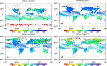
Figure 1 shows the global distribution of GEOS- XCO2 in 2010. GEOS- XCO2 had a clear seasonal cycle, a higher concentration of CO2 in the Northern Hemisphere winter and spring, e.g., concentrations in January and April are typically 385-390 ppm, and a CO2 concentration over the ocean of 381-385 ppm. Global CO2 concentrations were generally higher in June (383-388 ppm) than other months, and Northern Hemispheric CO2 concentrations were below those of the Southern Hemisphere in August. The GEOS- XCO2 over East Asia, Europe, eastern America, South America, and Central African equatorial regions was perennially high, possibly because fossil fuel combustion, biomass burning, and industrial emissions are more serious in these regions ( van der Werf et al., 2006). Therefore, in recent years, the increased concentration of CO2 may be mainly due to human activities in the Northern Hemisphere, but with a gradual spread from there to the Southern Hemisphere.
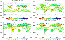
Figure 2 shows the distribution of GOSAT retrievals. Compared with the simulated spatial and temporal patterns of CO2 concentrations, the GOSAT CO2 products provide relatively few data. The polar regions having less data is mainly due to the effect of the viewing angle of the satellite sensor; when the solar zenith angle is greater than 75°, observations are considered to possess a higher level of error and are therefore filtered. In the tropics, missing data is due to there being more cloud and aerosols in this region; thus, during inversion, low-accuracy data are excluded. As can be seen from Fig. 2, the CO2 concentration over the oceans based on GOSAT satellite retrieval data varied from 380 to 385 ppm. The Northern Hemisphere in summer had a relatively low concentration of CO2, and the XCO2 in the terrestrial biosphere was generally lower than 377 ppm. The XCO2 over South America and the Southern Hemisphere as a whole was inconsistent, and the large deviations may have been due to the rainy season in the Amazon region, characterized by more cloud and aerosols, resulting in a lot of data being filtered out.
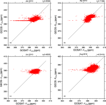
Finally in this section, we analyze the differences between the satellite retrievals and the model-simulated data. Figure 3 presents the differences between GOSAT- XCO2 and GEOS- XCO2 results for January, April, June, and August 2010. Data for the entire globe except some individual regions (e.g., over the Antarctic) are shown. GOSAT satellite retrieval data showed higher CO2 concentrations than the GEOS- XCO2 data. The differences over land areas in January and April ranged from 1 to 2 ppm, and there were major differences in June and August. For high-latitude regions in the Northern Hemisphere in June, as well as south of the Sahara, the difference was greater than 5 ppm, but with the model results showing higher concentrations than the GOSAT retrievals. In South America, meanwhile, the concentrations according to the satellite data were higher. The trend of the difference at high latitudes of the Northern Hemisphere and the Sahara region in August was opposite to June. The discrepancies between model-simulated results and satellite data in the polar and tropical regions, as well as near the Saharan region of Africa, the Amazon Basin, and some Asian regions were relatively large. These differences may have been caused by restrictions in the satellite sensors and algorithms. Figure 4 shows the correlation coefficients between the GOSAT observations and the GEOS- XCO2 simulation. As can be seen from the results, the maximum correlation coefficient in April reached 0.72. However, the correlation coefficients were smaller in June and August compared to April, and the correlation coefficient in January was only 0.36.
 | Figure 1 GEOS- XCO2 (ppm) global distribution in January, April, June, and August 2010. |
 | Figure 2 GOSAT retrieval data (ppm) distribution in January, April, June, and August 2010. |
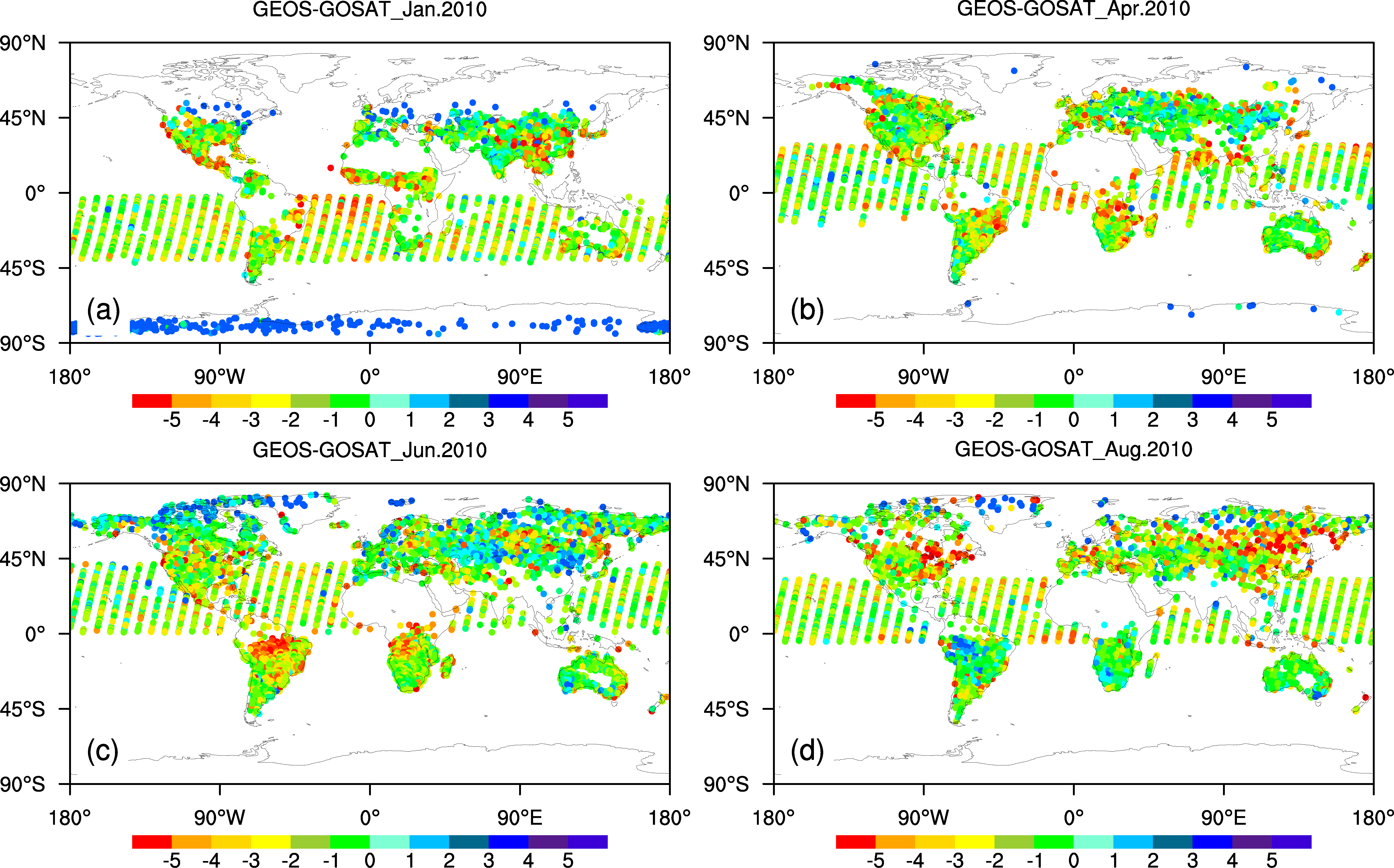 | Figure 3 Difference between GOSAT- XCO2 (ppm) and GEOS- XCO2 (ppm) in January, April, June, and August 2010. |
We also compared the XCO2 results from GEOS-Chem with TCCON data. It was found that the reasons for gaps between the GEOS- XCO2 and TCCON time series were clouds and instrumental issues. The number of coincident days between GEOS- XCO2 and TCCON data among stations varied from 23 (Ereka) to 291 (Lamont). The Lamont site had the largest number of coincident days because there were multiple orbit overpasses within the coincidence criteria and other sites had more cloud at these latitudes. The correlation coefficients in the Northern Hemisphere were higher than in the Southern Hemisphere (reaching 0.93 at Ny-Ålesund and Izana), but the correlation coefficient at Darwin in the Southern Hemisphere was only 0.42. The result was better than the comparison of the data from GEOS-Chem and GOSAT.
 | Figure 4 Correlation coefficients between GOSAT and GEOS- XCO2 data in January, April, June, and August 2010. |
The GEOS-Chem model can simulate the spatial and temporal distribution of the global atmospheric CO2 concentration, as well as the changes in global and regional atmospheric CO2 concentrations from real-time monitoring by satellites. However, because of restrictions in the sensor and inversion algorithms, we found that the atmospheric CO2 concentration has an inversion error of approximately 2 ppm. What needed to be verified was whether those data could reveal global and regional changes in atmospheric CO2 concentrations. We compared CO2 concentrations from GEOS-Chem and TCCON in this study, and found that the result was better than the comparison of data from GEOS-Chem and GOSAT. The correlation coefficients ranged from 0.42 to 0.92 (Table 1). In contrast to GOSAT and GEOS- XCO2, the difference over land areas in January and April was 1-2 ppm. Furthermore, a big difference was found in June and August. The difference in June was more than 5 ppm in high-latitude regions of the Northern Hemisphere, South America, and the Sahara Desert. In the high latitudes of the Northern Hemisphere, the data (CO2 concentrations) from the GEOS-Chem model simulations were higher than those from the GOSAT retrievals, while in South America the opposite was the case. The trend of the difference at high latitudes in the Northern Hemisphere and the Saharan region in August was opposite in June.
| Table 1 Coincident days and correlation coefficients ( r) between 14 Total Carbon Column Observing Network (TCCON) sites and model- simulated data. |
The retrieval accuracy of XCO2 has been continuously improved throughout the history of the development of the inversion algorithm based on the GOSAT XCO2 satellite. Currently, we have the advantage that the satellite can obtain data from anthropogenic emissions by source type in the refinement of the model simulation. Inversion data and effective model assimilation have become important ways to improve the accuracy of model simulations ( Zeng et al., 2013). At the same time, it is hoped that our work can help with preparations for a global CO2 data assimilation system.
Acknowledgments This work was supported by the National High Technology Research and Development Program of China (Grant No. 2013AA122002), the Knowledge Innovation Program of the Chinese Academy of Sciences (Grant No. KZCX2-EW-QN207), and the National Basic Research Program of China (Grant Nos. 2010CB428403 and 2009CB421407). In this article, TCCON data were obtained from the TCCON Data Archive, operated by the California Institute of Technology from the website at http://tccon.ipac.caltech.edu/, thanks for their support. We are also grateful to the ACOS and GOSAT teams for the availability of GOSAT observations and thank every member of these teams for their contributions to this study. Futhermore, Professors Liping LEI and Yi LIU are appreciated for their irreplaceable help for this paper.| 1 |
|
| 2 |
|
| 3 |
|
| 4 |
|
| 5 |
|
| 6 |
|
| 7 |
|
| 8 |
|
| 9 |
|
| 10 |
|
| 11 |
|
| 12 |
|
| 13 |
|
| 14 |
|