Stratospheric aerosols have an evident influence on the chemical and radiation balance of the atmosphere (e.g., McCormick et al., 1995; Hu and Shi, 1998; Solomon, 1999). Therefore, the ability to represent the distributional features of stratospheric aerosol is essential for a correct understanding and modeling of atmospheric processes. Additionally, stratospheric aerosols have been shown to be important in remote sensing retrievals. For example, to retrieve atmospheric trace gases and aerosol profiles from the limb observations of new-generation satellite systems, such as the Optical Spectrograph and Infrared Imager System (OSIRIS) ( Llewellyn et al., 2004) and the Scanning Imaging Absorption Spectrometer for Atmospheric Cartography (SCIAMACHY) system ( Bovensman et al., 1999), appropriate reference aerosol profiles are necessary in the retrieval calculation (e.g., Loughman et al., 2005; McLinden et al., 2010; Taha et al., 2011). Therefore, models of aerosol vertical distributions, which give realistic descriptions of an "average" atmosphere, are imperative both for the correct modeling of atmospheric processes and for accurate remote sensing retrievals.

In the past three decades, stratospheric aerosol has been intensively observed and studied (e.g., Lenoble and Brogniez, 1985; Trepte et al., 1994; Wang et al., 2004), with several climatologies and models of stratospheric aerosols having been proposed over different timescales (e.g., Brogniez and Lenobe, 1987; Hitchman et al., 1994; Kent et al., 1995; McCormick et al., 1993, 1996; Thomason et al., 1997; Bauman et al., 2003a, b; Bingen et al., 2004a, b). These climatologies and models provide valuable information on aerosol distributions in the stratosphere. However, these studies are mainly restricted to the altitudinal range below about 34 km. For the convenience of practical use, Fussen and Bingen (1999) proposed a reference model of the extinction coefficient of stratospheric aerosols on the basis of Stratospheric Aerosol and Gas Experiment (SAGE) II data. The basic variables of the model were the wavelength, latitude, relative altitude with respect to the tropopause, and a parameter that describes the volcanic status of the atmosphere. Based on the model of Fussen and Bingen (1999), Yang (2012) presented an empirical model for estimating background stratospheric aerosol extinctions over China. The results showed that this model can simulate well the aerosol distribution in the altitudinal range below about 33 km, but the estimated errors become larger at higher altitude levels. Therefore, further work is required in order to delineate aerosol distributions in the upper levels above 33 km and better describe aerosol distributions in the stratosphere under the volcanically quiescent conditions following the eruption of Mount Pinatubo.

In this context, the aim of this paper is to contribute to the characterization of the distribution of stratospheric aerosol by developing an empirical model for estimating the vertical distribution of aerosol extinction coefficients. The model will cover the latitudinal range between 60°S and 60°N and altitudes from 2 km above the tropopause to 40 km.

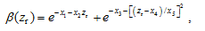
In this section, an empirical model for estimating the background stratospheric aerosol extinction profiles is created, on the basis of the zonal mean aerosol extinction profiles derived from the SAGE II measurements at 1.02, 0.525, and 0.452 μm. Analysis of aerosol vertical distribution features at different altitude levels shows that, although there are significant local-time variations in the vertical distribution of aerosol, the long-term averaged extinction profiles have regular features. Fussen and Bingen (1999) suggested an empirical expression to describe the vertical distribution of stratospheric aerosol extinction coefficients. The expression is in the form

, (1)

where

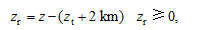(2)

and where β( z_r) is the aerosol extinction coefficient (km^-1) at the reduced altitude z_r, which is measured from 2 km above the tropopause; zis the altitude (km); z_t is the tropopause height (km); and x₁, x₂, x₃, x₄, x₅are fit coefficients related to the latitude. Starting at 2 km above the tropopause height avoids perturbations in the lowest levels of the stratosphere ( Brogniez and Lenobe, 1987). As described by Fussen and Bingen (1999) and Bingen and Fussen (2000), the first term of Eq. (1) stands for the aerosol's high-altitude exponential decrease behavior, and the second term represents a Gaussian peak centered at altitude x₄ with an amplitude exp ( x₃) and a width x₅ associated with the Junge layer.

Table 1

Table 1

Table 1 Empirical coefficients for calculating 1.02 μm aerosol extinction profiles used in Eq. (3). x1 x2 x3 x4 x5 50-60°N 8.63 0.258 9.81 6.0 5.86 40-50°N 8.90 0.263 9.73 5.0 6.40 30-40°N 9.79 0.243 9.63 2.0 6.92 20-30°N 9.88 0.310 9.77 1.0 8.12 10-20°N 9.58 0.440 9.77 3.6 7.31 0-10°N 9.80 0.430 9.66 3.8 7.50 0-10°S 9.80 0.430 9.67 3.9 7.50 10-20°S 9.58 0.440 9.77 3.7 7.29 20-30°S 9.87 0.300 9.79 1.1 8.10 30-40°S 9.90 0.250 9.58 2.3 6.93 40-50°S 8.90 0.263 9.77 5.9 6.32 50-60°S 8.63 0.258 9.84 6.7 5.80

Table 1 Empirical coefficients for calculating 1.02 μm aerosol extinction profiles used in Eq. (3).

Through numerical simulation and analysis, we discovered that the vertical distribution of aerosol extinction coefficients below about 33 km can be fitted well by this empirical expression, but at higher altitudes the biases become larger ( Yang, 2012). In order to better describe the aerosol distributional features at high altitudes above 33 km, we improved the above expression by adding a term. The improved expression is in the form

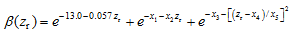, (3)

where all the variables are as already defined in Eq. (1). The first term in Eq. (3) mainly acts to simulate the aerosol profile in the upper levels. We chose the wavelength of 1.02 μm for the aerosol extinction profile calculation on the basis of Eq. (3). The empirical coefficients for each latitudinal band are determined empirically from a fit to the zonal mean aerosol extinction profiles derived from SAGE II measurements. In the calculation, the heights of the tropopause z_t are 10 km for 50-60°N and 50-60°S, 11 km for 40-50°N and 40-50°S, 14 km for 30-40°N and 30-40°S, and 16 km for the lower latitude bands in the tropics and subtropics. This calculation was carried out to 40 km. The five empirical coefficients derived using this expression are presented in Table 1. In practical use, the vertical distribution of stratospheric aerosol extinctions at 1.02 μm for each latitude band can be calculated according to Eq. (3) by employing these empirical coefficients.

In order to calculate aerosol extinction profiles at other wavelengths, we employed the expression suggested by Fussen and Bingen (1999), and express the aerosol extinction profile at the wavelength λas

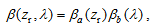, (4)

where β_a( z_r) is the 1.02 μm aerosol extinction coefficient at the reduced altitude z_r, and β_b( λ) is the dimensionless spectral dependence. As described by Fussen and Bingen (1999), this formal separation of the vertical and spectral dependence reflects the presence of a steep vertical structure of the aerosol layer and a smoother spectral dependence. The spectral dependence of the aerosol extinction coefficient is modeled by

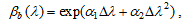(5)

where ∆ λ= λ-1.02 μm. This exponential dependence was proposed by Yue (1986), and was also used by Fussen and Bingen (1999). The advantages of this exponential formula are that it is the positive function and can describe the change of spectral behavior corresponding to all pos-sible stratospheric conditions. The parameters α₁ and α₂ in this formula are independent of the wavelength but dependent on the aerosol optical properties. Since the aerosol optical properties have vertical variations, the parameters α₁ and α₂ vary with the altitude, but this variation, as discussed by Fussen and Bingen (1999), is smaller than the variation described by β_b( λ). We found that the vertical distribution of α₁ and α₂ can be calculated by the following expressions:

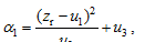, (6)

. (7)

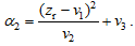
The empirical coefficients u₁, u₂, u₃and v₁, v₂, v₃ are determined empirically from a fit to the zonal mean SAGE II aerosol profiles at 1.02, 0.525, and 0.452 μm. The computation results are presented in Table 2. Using these coefficients, the spectral dependence β_b( λ) can be determined according to Eqs. (5)-(7), and then the extinction profile at the wavelength λcan be derived by employing Eq. (4). Note that this empirical model is restricted to extinction profile calculations in the visible and near-infrared range of the spectrum, since the spectral variation of aerosol extinction is quite smooth in this region and we based the calculations on the aerosol profile measurements at the wavelengths of 1.02, 0.525, and 0.452 μm.

Table 2

Table 2

Table 2 Empirical coefficients for calculating parameters α1 and α2 used in Eqs. (6) and (7). u1 u2 u3 v1 v2 v3 50-60°N 15.4 46.9 -4.6 13.3 27.5 -1.4 40-50°N 14.6 55.0 -4.3 12.0 30.0 -1.2 30-40°N 11.4 40.6 -4.1 9.3 24.0 -0.8 20-30°N 9.6 33.2 -4.0 8.0 18.3 -1.0 10-20°N 9.8 31.8 -3.7 8.4 17.0 -0.8 0-10°N 9.6 30.5 -3.8 8.4 15.6 -1.3 0-10°S 10.1 30.3 -4.0 8.7 16.3 -1.5 10-20°S 9.5 28.3 -4.1 8.1 15.6 -1.5 20-30°S 8.9 25.8 -4.6 7.6 15.0 -2.1 30-40°S 11.2 33.3 -4.9 9.3 19.6 -2.2 40-50°S 13.0 54.0 -4.7 10.3 30.5 -2.1 50-60°S 15.1 62.4 -4.6 12.1 38.8 -1.4

Table 2 Empirical coefficients for calculating parameters α1 and α2 used in Eqs. (6) and (7).

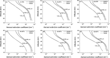
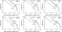
Figures 1 and 2 show comparisons of model-calculated and SAGE II-measured zonal mean aerosol extinction profiles at the wavelengths of 1.02, 0.525, and 0.452 μm for each latitude band in the Northern and Southern Hemisphere, respectively. As shown in Figs. 1 and 2, for all the wavelengths and latitudes, the model-calculated aerosol extinction coefficients generally agree well with the SAGE II values. The smooth curves (dashed lines) derived from the model estimation can simulate well the actual SAGE II-measured zonal mean extinction profiles (solid lines). The relative differences between the model- calculated and the corresponding SAGE II-measured aerosol extinction coefficients are generally within 15% from 2 km above the tropopause to 40 km.

Figure 1

	Figure Option ViewDownloadNew Window
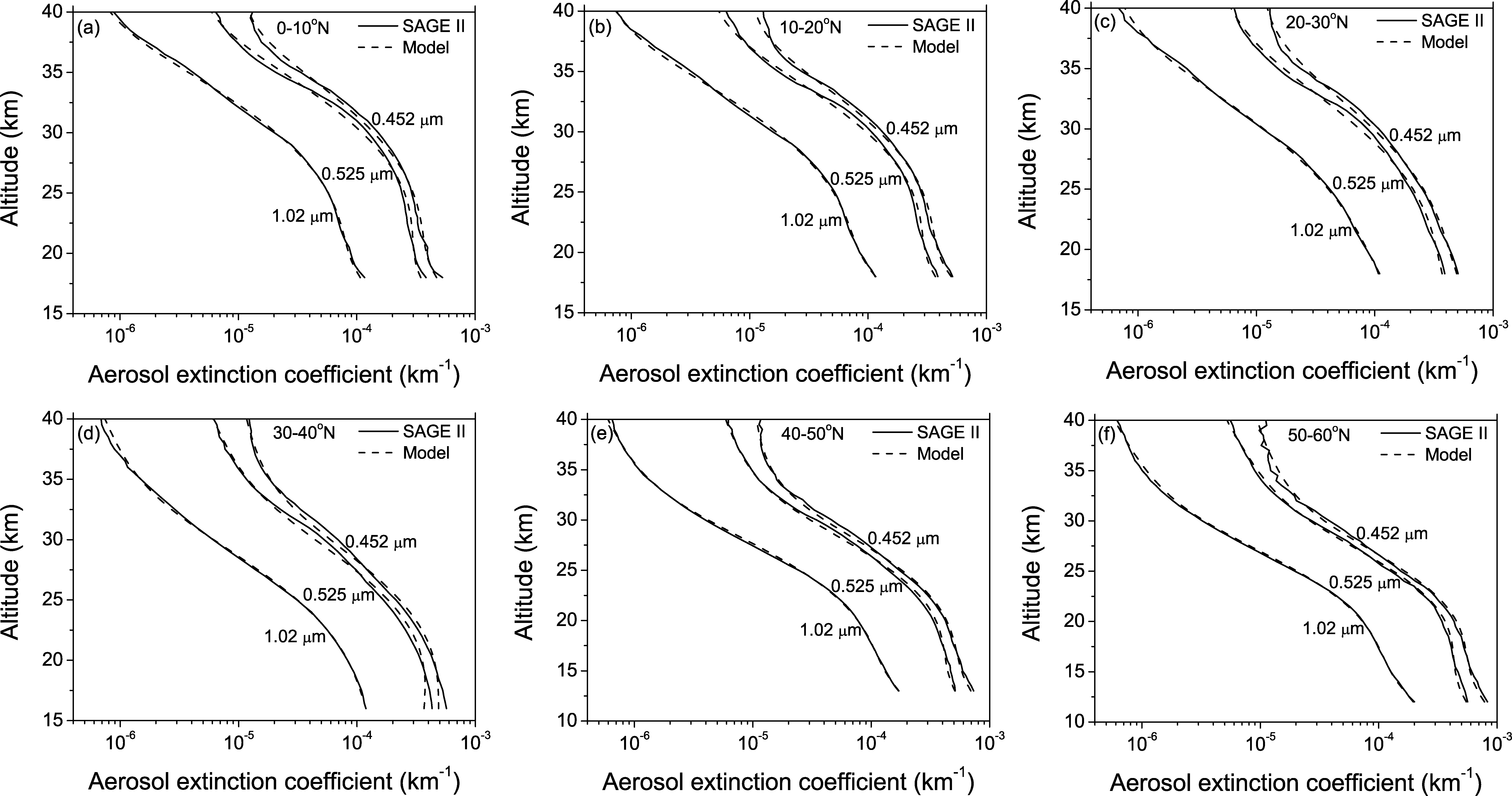	Figure 1 Comparisons of model-calculated and SAGE II-measured zonal mean aerosol extinction profiles at the wavelengths of 1.02, 0.525, and 0.452 μm for each latitude band in the Northern Hemisphere.

Figure 2

	Figure Option ViewDownloadNew Window
	Figure 2 Comparisons of model-calculated and SAGE II-measured zonal mean aerosol extinction profiles at the wavelengths of 1.02, 0.525, and 0.452 μm for each latitude band in the Southern Hemisphere.

For quantitative comparisons, the quantity of model- calculated and SAGE II-measured aerosol optical depths (vertically integrated aerosol extinction coefficient) for different altitude levels are compared. Tables 3-5 present comparisons of the zonal mean aerosol optical depths from 2 km above the tropopause ( H_T+2) to 5 km above the tropopause ( H_T+5), H_T+5 to 40 km, and H_T+2to 40 km for each latitude band at the wavelengths of 1.02, 0.525, and 0.452 μm, respectively. It can be seen from the results presented in Tables 3-5 that there is good agreement between the model-calculated optical depths and the corresponding optical depths derived from SAGE II measurements. The relative differences are within 9% in the lower altitude region from H_T+2 to H_T+5, within 4.6% from H_T+5 to 40 km, and within 0.9% from H_T+2 to 40 km. The comparison results show that the model prediction of aerosol optical depths can represent well a reasonable average of the SAGE II observational values across the altitude range from H_T+2 to 40 km.

Table 3

Table 3

Table 3 Comparisons of model-calculated and SAGE II-measured 1.02 μm aerosol optical depths ( multiplied by 1000) within the altitude range from 2 km above the tropopause ( HT+2) to 5 km above the tropopause ( HT+5), HT+5 to 40 km, and HT+2 to 40 km for each latitude band. The zonal mean tropopause heights ( HT) for each latitude band are also given. HT(km) HT+2- HT+5 HT+5- 40 km HT+2- 40 km SAGE II Model Dif (%) SAGE II Model Dif (%) SAGE II Model Dif (%) 50-60°N 10.0 0.475 0.472 -0.63 0.779 0.781 0.26 1.254 1.253 -0.08 40-50°N 11.0 0.424 0.421 -0.71 0.711 0.713 0.28 1.135 1.134 -0.09 30-40°N 14.0 0.323 0.319 -1.24 0.468 0.472 0.85 0.791 0.791 0.00 20-30°N 16.0 0.273 0.275 0.73 0.389 0.386 -0.77 0.662 0.661 -0.15 10-20°N 16.0 0.279 0.278 -0.36 0.468 0.468 0.00 0.747 0.746 -0.13 0-10°N 16.0 0.283 0.272 -3.89 0.527 0.532 0.95 0.810 0.804 -0.74 0-10°S 16.0 0.266 0.269 1.13 0.532 0.534 0.38 0.798 0.803 0.63 10-20°S 16.0 0.267 0.276 3.37 0.481 0.473 -1.66 0.748 0.749 0.13 20-30°S 16.0 0.271 0.274 1.11 0.399 0.390 -2.26 0.670 0.664 -0.90 30-40°S 14.0 0.295 0.314 6.44 0.515 0.494 -4.08 0.810 0.808 -0.25 40-50°S 11.0 0.363 0.395 8.82 0.769 0.735 -4.42 1.132 1.130 -0.18 50-60°S 10.0 0.424 0.452 6.60 0.822 0.792 -3.65 1.246 1.244 -0.16 Note: Dif (%) = (model-calculated - SAGE II-measured)/SAGE II measured×100.

Table 3 Comparisons of model-calculated and SAGE II-measured 1.02 μm aerosol optical depths ( multiplied by 1000) within the altitude range from 2 km above the tropopause ( HT+2) to 5 km above the tropopause ( HT+5), HT+5 to 40 km, and HT+2 to 40 km for each latitude band. The zonal mean tropopause heights ( HT) for each latitude band are also given.

Table 4

Table 4

Table 4 Comparisons of model-calculated and SAGE II-measured 0.525 μm aerosol optical depths ( multiplied by 1000) within HT+2 to HT+5, HT+5 to 40 km, and HT+2 to 40 km for each latitude band. HT for each latitude band are also given. HT(km) HT+2- HT+5 HT+5- 40 km HT+2- 40 km SAGE II Model Dif (%) SAGE II Model Dif (%) SAGE II Model Dif (%) 50-60°N 10.0 1.551 1.455 -6.19 3.661 3.767 2.90 5.212 5.222 0.19 40-50°N 11.0 1.442 1.377 -4.51 3.259 3.346 2.67 4.701 4.723 0.47 30-40°N 14.0 1.218 1.119 -8.13 2.321 2.427 4.57 3.539 3.546 0.20 20-30°N 16.0 1.053 1.027 -2.47 1.963 1.996 1.68 3.016 3.023 0.23 10-20°N 16.0 1.000 0.963 -3.70 2.192 2.215 1.05 3.192 3.178 -0.44 0-10°N 16.0 0.971 0.943 -2.88 2.373 2.402 1.22 3.344 3.345 0.03 0-10°S 16.0 0.925 0.875 -5.41 2.390 2.446 2.34 3.315 3.321 0.18 10-20°S 16.0 0.982 0.936 -4.68 2.253 2.299 2.04 3.235 3.235 0.00 20-30°S 16.0 1.065 1.019 -4.32 2.031 2.087 2.76 3.096 3.106 0.32 30-40°S 14.0 1.168 1.089 -6.76 2.570 2.645 2.92 3.738 3.734 -0.11 40-50°S 11.0 1.352 1.333 -1.41 3.644 3.672 0.77 4.996 5.005 0.18 50-60°S 10.0 1.475 1.453 -1.49 3.972 4.003 0.78 5.447 5.456 0.17

Table 4 Comparisons of model-calculated and SAGE II-measured 0.525 μm aerosol optical depths ( multiplied by 1000) within HT+2 to HT+5, HT+5 to 40 km, and HT+2 to 40 km for each latitude band. HT for each latitude band are also given.

Table 5

Table 5

Table 5 Comparisons of model-calculated and SAGE II-measured 0.452 μm aerosol optical depths ( multiplied by 1000) within HT+2 to HT+5, HT+5 to 40 km, and HT+2 to 40 km for each latitude band. HT for each latitude band are also given. HT(km) HT+2- HT+5 HT+5- 40 km HT+2- 40 km SAGE II Model Dif (%) SAGE II Model Dif (%) SAGE II Model Dif (%) 50-60°N 10.0 2.133 2.007 -5.91 4.675 4.795 2.57 6.808 6.802 -0.09 40-50°N 11.0 1.903 1.822 -4.26 4.124 4.193 1.67 6.027 6.015 -0.20 30-40°N 14.0 1.572 1.449 -7.82 2.989 3.093 3.48 4.561 4.542 -0.42 20-30°N 16.0 1.347 1.321 -1.93 2.507 2.527 0.80 3.854 3.848 -0.16 10-20°N 16.0 1.302 1.262 -3.07 2.763 2.795 1.16 4.065 4.057 -0.20 0-10°N 16.0 1.257 1.223 -2.70 2.937 2.960 0.78 4.194 4.183 -0.26 0-10°S 16.0 1.181 1.121 -5.08 2.947 2.995 1.63 4.128 4.116 -0.29 10-20°S 16.0 1.224 1.187 -3.02 2.781 2.838 2.05 4.005 4.025 0.50 20-30°S 16.0 1.308 1.261 -3.59 2.522 2.551 1.15 3.830 3.812 -0.47 30-40°S 14.0 1.418 1.361 -4.02 3.169 3.219 1.58 4.587 4.580 -0.15 40-50°S 11.0 1.622 1.628 0.37 4.420 4.403 -0.38 6.042 6.031 -0.18 50-60°S 10.0 1.895 1.842 -2.80 4.933 4.972 0.79 6.828 6.814 -0.21

Table 5 Comparisons of model-calculated and SAGE II-measured 0.452 μm aerosol optical depths ( multiplied by 1000) within HT+2 to HT+5, HT+5 to 40 km, and HT+2 to 40 km for each latitude band. HT for each latitude band are also given.

In this paper, we have presented an empirical model for estimating the vertical distribution of background stratospheric aerosol extinction coefficients on the basis of SAGE II aerosol extinction profile data at 1.02, 0.525, and 0.452 μm during the period 1998-2004. Comparisons have shown that the model-calculated aerosol extinction profiles conform well with the SAGE II measurements, with the relative difference generally being within 15% from 2 km above the tropopause to 40 km. Comparisons have also shown that the model-calculated aerosol optical depths are in very good agreement with the corresponding SAGE II values, with the relative differences being within 0.9% for all latitude bands. The model developed in this paper can be used in atmospheric modeling and remote sensing retrievals. However, considering that the stratospheric aerosol distribution is affected by the perturbations of volcanic eruptions and circulation variations, the exact shape of the aerosol profile in different locations is still rather unknown. Therefore, in some practical uses, such as climatological trend analysis, this model is not applicable, and the variability of aerosol distribution needs to be taken into account.

Acknowledgments. The authors wish to acknowledge the National Aeronautics and Space Administration (NASA) Langley Research Center for the SAGE II aerosol data. This work was supported by the National Natural Science Foundation of China (Grant No. 41275047), the National Basic Research Program of China (Grant No. 2013CB955801), and the Strategic Priority Research Program of the Chinese Academy of Sciences (Grant No. XDA05100300).