
A Numerical Verification of Self-Similar Multiplicative Theory for Small-Scale Atmospheric Turbulent Convection
[SONG Zong-Peng1, 2 , HU Fei1  , LIU Yu-Jue
1, 2 , CHENG Xue-Ling1 , LIU Lei1 , XU Jing-Jing1 ]
, LIU Yu-Jue|
|


The self-similar multiplicative theory (SSM theory), aims to interpret the scaling behavior of the temperature structure function. In the present paper, the author report results from a numerical simulation of atmospheric turbulent convection in order to verify this theory. The simulation was based on a shell model which was deduced from simplified atmospheric convection equations. The numerical results agreed well with the theory prediction of scaling law from the first order to the eighth order. They also showed that the prediction of this theory was better than that given by the Kolmogorov’s theory in 1941, log-normal, and
Small-scale (homogeneous isotropic) turbulent convection is important to the diffusion process and the universal similarity laws ( Katul et al., 2011) in the atmospheric boundary layer. Usually, the temperature structure function is used to study the statistical properties of turbulent convection, which is the statistical average of the moments of temperature fluctuations on spatial scales. Experiments have shown that the temperature structure function is proportional to the power of the spatial scale in the inertial range ( Frish, 1995; Lohse and Xia, 2010). There has been much debate on the power exponents of the temperature structure function. Kolmogorov’s theory ( Kolmogorov, 1941; Corrsin, 1951) predicts a linear relation, which is called the K41 scaling law. However, there are plenty of experimental results ( Antonia et al., 1984; Frish, 1995; Ruiz-Chavarria et al., 1996) that deviate from the K41 scaling law. To correct K41, Antonia et al. (1984) gave two predictions of scaling law according to the log-normal theory ( Kolmogorov, 1962; Obukhov, 1962) and β model theory ( Frish et al., 1978), which we show in section 3.
Hu (1995) proposed an improved theory—the self- similar multiplicative theory (SSM theory). This theory assumes the scaling ratio of energy at different scales is similar, and temperature fluctuations obey an exponential distribution. The SSM theory improved the prediction of the scaling law, and this improved scaling law was proved to be valid in an experiment by Hu et al. (2005).
In the present paper, we report results from a numerical simulation of small-scale atmospheric turbulent convection, and use the numerical data to verify the scaling law predicted by the SSM theory. The numerical simulation was based on a shell model, which was deduced from simplified atmospheric convection equations ( Liu et al., 1996). We state the principle of the shell model in section 2. In section 3, the computed power exponents of the structure function on the numerical data are presented, and then a comparison is made between the numerical and experimental results to verify the appropriateness of the numerical data. Next, we compare the numerical results and the four scaling laws, in which we focus on the numerical verification of the scaling law predicted by the SSM theory. In addition, we also computed the thermal energy spectrum andprobability distribution functions (PDFs) of temperature fluctuation, the results of which are also reported in section 3. Finally, the major conclusions of the study are summarized in section 4.
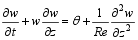
Numerical simulation is a common research tool for the study of turbulence. However, a direct simulation of atmospheric turbulent convection consumes much computing resource. A shell model consumes much less computing resource. Although it is a reduced simulation model, many statistical properties are still preserved well ( Gledzer, 1973; Yamada and Ohkitani, 1987). Shell models have been used to study homogeneous isotropic turbulence for computing the power exponents of the structure function, energy spectrum, and PDFs of temperature (or velocity) fluctuation ( Brandenburg, 1992; Ching and Cheng, 2008). The shell model was developed from the atmospheric convection equations. According to Liu et al. (1996), atmospheric convection equations can be simplified by neglecting the horizontal velocity in the momentum equation and the heat transport equation:
 | , (1) |
 | (2) |
where z, w, and θ are dimensionless vertical height, vertical velocity, and potential temperature; z, w, and θare non-dimensionalized with characteristic vertical length, characteristic vertical velocity, and characteristic potential temperature, respectively. Re, Ri, and Pr are the Reynolds number, the bulk Richardson number, and the Prandtl number, respectively. For the Rayleigh number, Ra, a dimensional analysis gives the following relation:

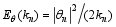
A shell model is constructed in wavenumber space. Wavenumber space is divided into spherical shells, each assigned a wavenumber, kn, which is the radius of the sphere, kn= k0 qn, k0is the initial wavenumber, qis a controllable parameter, and n =1, 2, …, N. The vertical velocity and temperature on the nth shell are expressed by a set of complex variables, { wn = wn+ iwn} and { θn= θn+ iθn}. The physical meaning of wn and θn are velocity fluctuation, δ w( rn), and temperature fluctuation, δ θ( rn), at the spatial scale, rn( rn~1 /kn). The kinetic energy, thermal energy, and their energy spectrums are defined as 


According to Eqs. (1) and (2), and the above hypothesis, the equations of the shell model are adapted as
 | (4) |
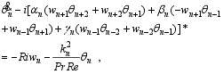 | (5) |
where the asterisk (*) refers to the complex conjugate, and the overdot (˙) refers to a time derivative.
The real constants, an, bn, cn, αn, βn, and γn, are defined as
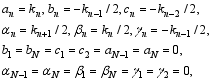 | (6) |
so that the nonlinear terms of Eqs. (4) and (5) conserve the kinetic energy, Ek, and thermal energy, Eθ, respectively.
Parameters were assigned as: k0 = 0.2, q = 2, N = 24. Because z is non-dimensionalized by the characteristic vertical length, the physical scale of the wavenumber relies on the characteristic vertical length. If the characteristic vertical length is 1500 m (the height of atmospheric boundary layer), the physical scale of the initial wavenumber, k0, and the end wavenumber, k24, are about 50 m and 3 μm, respectively. Re = 1.4 × 10⁷, Pr = 0.70, Ri = -0.0001 . According to Eq. (3), the Ra for this computation is 1.0 × 10¹⁰. To integrate the ordinary differential Eqs. (4) and (5), we employed the Gauss method. We integrated for each time interval, h = 10-7s. The initial condition of the numerical integration was chosen as 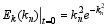

The pth order power exponents, ξp, of the structure function on the numerical data were computed. The structure function is the statistical average of pth order moments of the temperature differences, δ θ( r), on the spatial scale, r. In a shell model, the physical meaning of θn is the temperature fluctuation, δ θ( rn), at the spatial scale, rn ( rn~1 /kn). Therefore, the temperature structure function can be written as <| θn| p>. Because the temperature structure function, <| θn| p>, is proportional to the power of scale rn ( rn~1 /kn), we obtained <| θn| p>∝ 
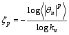
Computed by the above method, ξp is the absolute power exponent. We used the extended self-similarity method (ESS) ( Benzi et al., 1995) to compute the relative power exponent rather than absolute power exponent. ESS can enhance the computation accuracy. We chose ξp/ξ4 as the relative scaling, 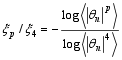
In experiments ( Warhaft, 2002; Hu et al., 2005; Sun et al., 2006; Lohse and Xia, 2010), ξ4 is very close to 1. Therefore, we considered that the absolute power exponent, ξp, equals the relative power exponent, ξp/ξ4.
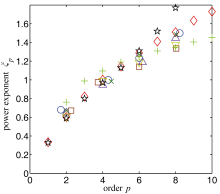
By applying the ESS method to the numerical data, we obtained ξp, as shown by the diamond symbol in Fig. 1. Figure 1 also shows experimental results for comparison. Experiments were carried out under different circumstances. Theoretically, the experimental results should have been universal, but in reality they were not. In addition to systematic error, they may also have been subject to external circumstances that affected the results and caused differences. Although the experimental results were different from each other, they shared the same trend. The numerical results followed this trend, and were within the discrepancy range of the experimental results.
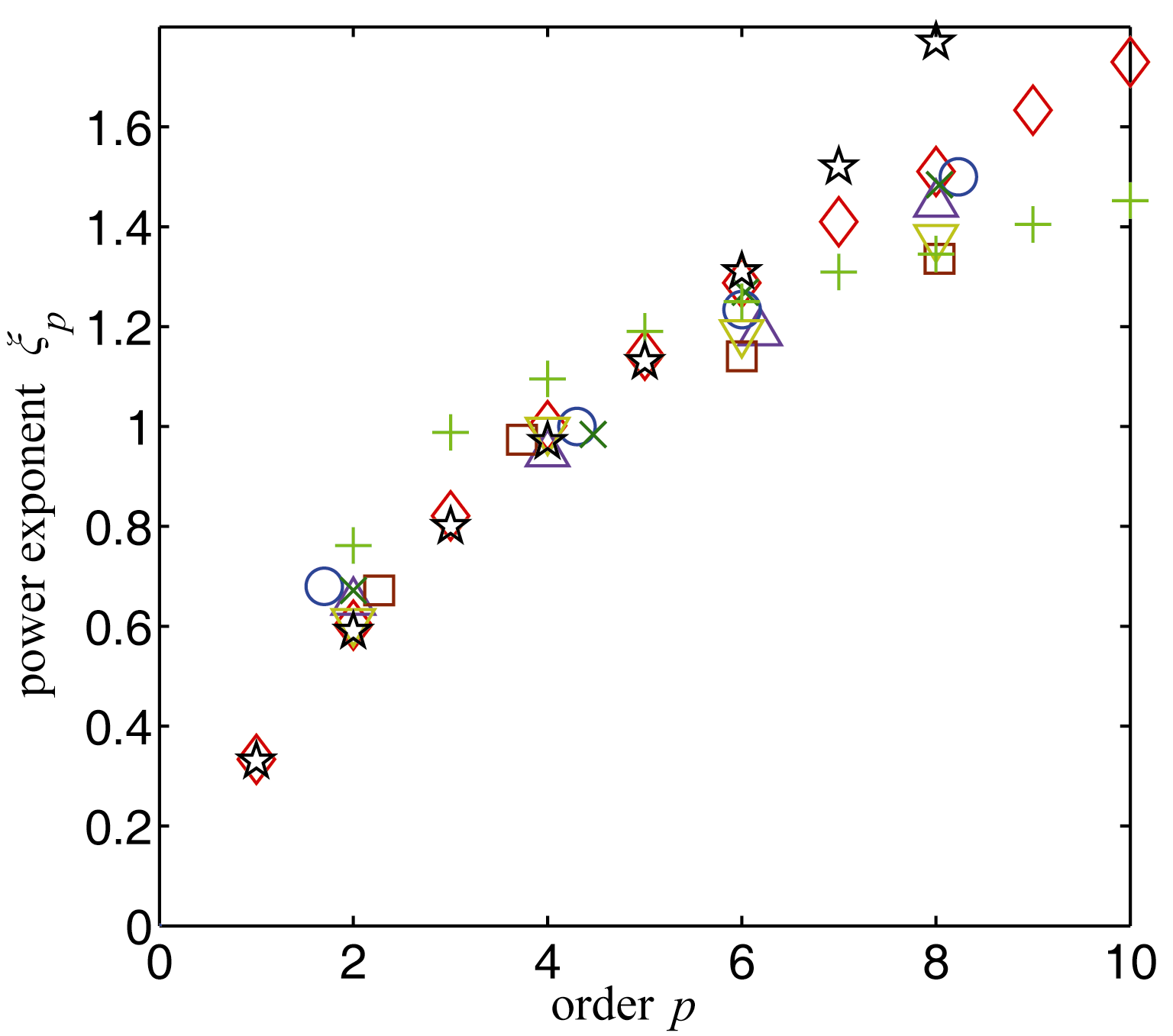 | Figure 1 The power exponent ( ξp) from different sources: (◇) our numerical simulation; (+) urban canopy layer experiment ( Hu et al., 2005); (□) atmospheric surface layer over ocean ( Antonia et al., 1984); (×) atmospheric surface layer over land ( Antonia and Van Atta, 1978); (▽) boundary layer ( Antonia et al., 1984); (○) round jet 1 ( Antonia and Van Atta, 1978); (△) round jet 2 ( Antonia et al., 1984); (☆) laboratory convection cell, sidewall data ( Sun et al., 2006). |
This is the most important part of the paper. The numerical results of ξp were compared with four scaling laws. We focused on the verification of the scaling law predicted by the SSM theory. In Fig. 2, the diamond symbol refers to the numerical results for ξp; line I is the scaling law predicted by the K41 theory: ξp = p/3 ( Kolmogorov, 1941; Corrsin, 1951); line II is the scaling law predicted by the β model theory: ξp = p/3 + μ(3- p)/3, where μ is the intermittent parameter and equals 0.2 ( Frish et al., 1978; Antonia et al., 1984); line III is the scaling law predicted by the log-normal theory: ξp = p/3- μp [(10-6 ρ) p-12]/72, where ρ is the statistical correlation parameter and equals 0.5, and μ equals 0.2 ( Kolmogorov, 1962; Obukhov, 1962; Antonia et al., 1984); line IV is the scaling law predicted by the SSM theory: ξp = p/3- μ[ p( p +6)/72 + (2ln p!- pln2)/2ln6], where μ equals 0.2 ( Hu, 1995).
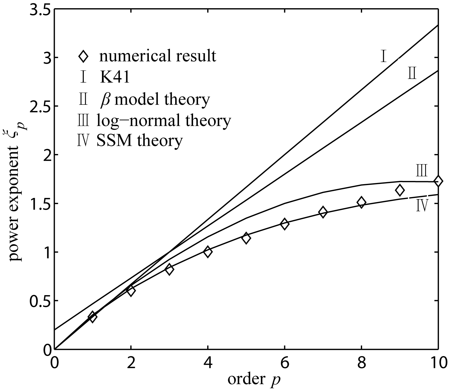 | Figure 2 Comparison of the numerical results of ξp with scaling laws predicted by theories. |
From Fig. 2, it can be seen that the scaling law predicted by the SSM theory was highly consistent with the numerical results from the first to the eighth order, and it was better than the K41, log-normal, and β model theories. The numerical results offer strong support for the SSM theory.
In addition, we calculated the errors between the four scaling laws and the experimental results (including thenumerical results), and these are shown in Table 1. Errors are the average relative errors of all orders of the power exponents, ξp. We can see that the error in the SSM theory was obviously smaller than that of the others. The prediction of the SSM theory was better than that given by the K41, βmodel, and log-normal theories.
| Table 1 Errors between four scaling laws predicted by theories and experimental results. |
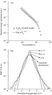
Energy spectrum and PDFs are very important in atmospheric turbulence research. Although they are not the emphasis of this paper, we still computed them for added interest. As mentioned before, the thermal energy spectrum, Eθ( kn), equals | θ|2/(2 kn). PDFs are probability distribution functions of the temperature fluctuation, θn, at spatial scale, rn. These were computed and the results are shown in Fig. 3. As shown in Fig. 3a, Eθ( kn) (diamond symbol) obeys Kolmogorov’s -5/3 law (solid line) in the inertial range and damps at large wavenumbers. The experimental results were almost the same as the numerical results, except for a “bump” at high wavenumbers approaching the dissipation range ( Hill, 1978). In Fig. 3b, it can be seen that these PDFs have exponential tails that are obviously different from the Gaussian distribution. The PDFs at the smaller scale have longer tails than those at the larger scale. These results are very consistent with previous reported experimental results ( Lohse and Xia, 2010; Quan et al., 2007).
 | Figure 3 Numerical results: (a) thermal energy spectrum Eθ(kn); (b) normalized PDFs of the temperature fluctuation, θn/ σ, at spatial scale, rn, where σ is the standard deviation and n = 6, 11, 17. A larger value of n corresponds to the smaller scale, and a smaller value of n corresponds to the bigger scale. Here we show the real part of the temperature. Physical quantities here are all dimensionless, which was declared in section 2 . |
A shell model was adapted to simulate small-scale atmospheric turbulent convection. Numerical results were used to verify the scaling law predicted by the SSM theory. The numerical results were found to be reliable upon examination, and highly consistent with the prediction of the orders p = 1, 2, 3, …, 8, offering strong support for the SSM theory. Other experimental results did not agree as well with the SSM theory as the numerical results did. However, the results based on SSM theory still fitted better than those of the K41, log-normal, and βmodel theories.
Although the SSM theory results fitted perfectly with the first eight orders, they deviated from the numerical results when exceeding the eighth order. The discrepancy grew larger as p increased. We also found the same situation when fitting the experimental results. In addition, as we see in Fig. 1, the experimental results were different from each other. This discrepancy may have been caused by the changing of parameter Ra. In our simulation, we also found that ξp changed with Ra. We argue that different Ra results in a different degree of intermittence of turbulent fluctuation. Therefore, there exists some relationship between Ra and μ. Although the SSM theory could make up the discrepancy by changing the intermittent parameter, μ, it cannot explain the relation between μ and Ra. More in-depth study is needed to perfect this theory.
Acknowledgements. The authors appreciate the contribution to this article from Dr. Jiong CHEN. This work was supported by the strategy guide for the specific task of the Chinese Academy of Sciences: Carbon-budget Certification to Deal with Climate Change and Relevant Issues (Grant No. XDA05000000), its sub program: Big Tower Certification System and Comprehensive Observation (Grant No. XDA05040301), and Shenzhen Bureau of Meteorology.
| 1 |
|
| 2 |
|
| 3 |
|
| 4 |
|
| 5 |
|
| 6 |
|
| 7 |
|
| 8 |
|
| 9 |
|
| 10 |
|
| 11 |
|
| 12 |
|
| 13 |
|
| 14 |
|
| 15 |
|
| 16 |
|
| 17 |
|
| 18 |
|
| 19 |
|
| 20 |
|
| 21 |
|
| 22 |
|
| 23 |
|