
Understanding the Global Surface-Atmosphere Energy Balance in FGOALS-s2 through an Attribution Analysis of the Global Temperature Biases
[YANG Yang1, 2 , REN Rong-Cai1, *  ]
]
]
|
|


Citation: Yang, Y., and R.-C. Ren, 2015: Understanding the global surface-atmosphere energy balance in FGOALS-s2 through an attribution analysis of the global temperature biases, Atmos Oceanic Sci. Lett., 8, 107-112.
doi:10.3878/AOSL20150019.
Received:6 February 2015; revised:9 March 2015; accepted:11 March 2015; published:16 March 2015
Based on an attribution analysis of the global mean temperature biases in the Flexible Global Ocean- Atmosphere-Land System model, spectral version 2 (FGOALS-s2) through a coupled atmosphere-surface climate feedback-response analysis method (CFRAM), the model’s global surface-atmosphere energy balance in boreal winter and summer is examined. Within the energy-balance-based CFRAM system, the model temperature biases are attributed to energy perturbations resulting from model biases in individual radiative and non-radiative processes in the atmosphere and at the surface. The results show that, although the global mean surface temperature ( Ts) bias is only 0.38 K in January and 1.70 K in July, and the atmospheric temperature ( Ta) biases from the troposphere to the stratosphere are only around ±3 K at most, the temperature biases due to model biases in representing the individual radiative and non-radiative processes are considerably large (over ±10 K at most). Specifically, the global cold radiative Ts bias, mainly due to the overestimated surface albedo, is compensated for by the global warm non-radiative Ts bias that is mainly due to the overestimated downward surface heat fluxes. The model biases in non-radiative processes in the lower troposphere (up to 5-15 K) are relatively much larger than in upper levels, which are mainly responsible for the warm Ta biases there. In contrast, the global mean cold Ta biases in the mid-to-upper troposphere are mainly dominated by radiative processes. The warm/cold Ta biases in the lower/upper stratosphere are dominated by non-radiative processes, while the warm Ta biases in the mid-stratosphere can be attributed to the radiative ozone feedback process.
The global mean temperature is one of the most critical metrics for assessing climate variabilities and climate changes. It can broadly indicate the changes in other climate variables such as precipitation extremes, global sea level, water vapor content, and the lapse rate of the atmosphere. It also reflects the effects of cloud fraction feedbacks, the phase of atmospheric carbon dioxide, and changes in atmospheric circulations (Colman, 2001; Kharin et al., 2007; Vermeer and Rahmstorf, 2009; Butler et al., 2010; Humlum et al., 2013). A model’ s reproducibility of the observed global mean surface and atmospheric temperature and its changes is an important measure of its performance in simulating the climate system and climate changes.
It is known that most current models suffer from considerable temperature biases at the surface (Ts) and in the atmosphere (Ta) across the globe. The model biases in FGOALS-s2 (the Flexible Global Ocean-Atmosphere- Land System model, spectral version 2) with respect to sea surface temperature (Lin et al., 2013), and that in the troposphere and stratosphere (Ren et al., 2009; Ren and Yang, 2012), and the exaggerated warming response to anthropogenic forcing (Zhou et al. 2013), have been investigated in numerous previous studies.
The model biases in global meanTs and Ta are largely associated with the global energy balance among the various physical processes including radiative processes (e.g., cloud, albedo feedbacks) and non-radiative processes (e.g., surface turbulent fluxes and large-scale circulation) within the model climate system (Randall et al., 2007). It is critically important to understand the global temperature biases in a framework of energy balance.
Recently, based on the energy balance within each surface-atmosphere column, Lu and Cai (2009) and Cai and Lu (2009) developed a coupled atmosphere-surface climate feedback-response analysis method (CFRAM), which was originally developed for quantitative evaluation of the climate feedbacks to global warming (Lu and Cai, 2010; Cai and Tung, 2012). In this process-based decomposition framework, the temperature difference between two climate states can be attributed to individual physical processes, including radiative processes (e.g., external forcing, ozone, water vapor, cloud, and surface albedo feedback) and non-radiative processes (e.g., surface sensible/latent heat fluxes and dynamic processes in the atmosphere and at the surface). By adopting the CFRAM, the surface temperature biases in version 1 of the Community Earth System Model (CESM1) (Park et al., 2014) and the surface and atmospheric temperature biases in FGOALS-s2 (Yang et al., 2015; Ren et al., 2015) have been dissected and quantitatively attributed to various radiative and non-radiative processes. It was indicated that, unlike that in CESM1, where radiative processes such as albedo feedback are important contributors, the Ts biases in FGOALS-s2 are largely due to the model bias in non-radiative processes such as surface heat fluxes. The Ts biases in FGOALS-s2 are relatively larger over land than over the oceans, and larger in boreal summer than in boreal winter. The model temperature biases in the atmosphere were also attributed to model biases in radiative or non-radiative processes in different latitudinal bands (Ren et al., 2015).
In this study, we aim to provide a global or zonal-mean overview of, rather than detailed local information on, the energy balance in FGOALS-s2 through an attribution analysis of the Ts and Ta biases in the model with respect to reanalysis data. To do so, we use the process-based decomposition method, CFRAM, a coupled surface-atmosphere energy balance system. The purpose of the study is to further understand the general features of the model biases and the physical processes that are responsible, and ultimately provide useful information for future improvements of the model.
The remainder of the paper is organized as follows: Section 2 briefly introduces the data used, the FGOALS- s2 model, and the CFRAM method. Section 3 presents the main results. A summary is provided in section 4.
FGOALS-s2 is one of the member models of the Coupled Model Intercomparison Project Phase 5 (CMIP5). Its atmospheric component is version 2 of the Spectral Atmospheric Model of the State Key Laboratory of Numerical Modeling for Atmospheric Sciences and Geophysical Fluid Dynamics (LASG), Institute of Atmospheric Physics (IAP) (SAMIL2) (Wu et al., 1996), with a horizontal resolution of R42 (approximately 1.66° (latitude) × 2.81° (longitude)), and 26 vertical levels. The oceanic component is version 2 of the LASG/IAP Climate Ocean Model (LICOM2), with a 1° resolution in the horizontal direction (0.5° meridional resolution in the tropics), and 30 vertical levels (Liu et al., 2012). The land and sea ice components are version 3 of the Community Land Model (CLM3) (Oleson et al., 2004) and version 5 of the Community Sea Ice Model (CSIM5) (Briegleb et al., 2004), respectively. The four components are coupled through a flux coupler (Collins et al., 2006). More detailed descriptions of the model can be found in Bao et al. (2013).
The European Center for Medium-Range Weather Forecasts (ECMWF) Re-Analysis Interim (ERA-Interim) dataset (Dee et al., 2011) covers the period from 1979 to the present day, with a horizontal resolution of 1.5° (longitude) × 1.5° (latitude) and 37 pressure levels from 1000 to 1 hPa. The CMIP5 historical run of FGOALS-s2 covers the period from 1850 to 2005. The model biases are defined as the differences in the climatological mean fields between FGOALS-s2 and ERA-Interim during 1979- 2005.
Based on the energy balance within a multi-layer surface-atmosphere column, the difference (
where
where
Substituting Eqs. (2)-(4) into Eq. (1), and rearranging the terms and multiplying both sides of the resultant equation by
Equation (5) states that the local temperature difference (including Ts and Ta) at each grid point between FGOALS-s2 and ERA-Interim (
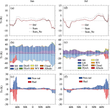
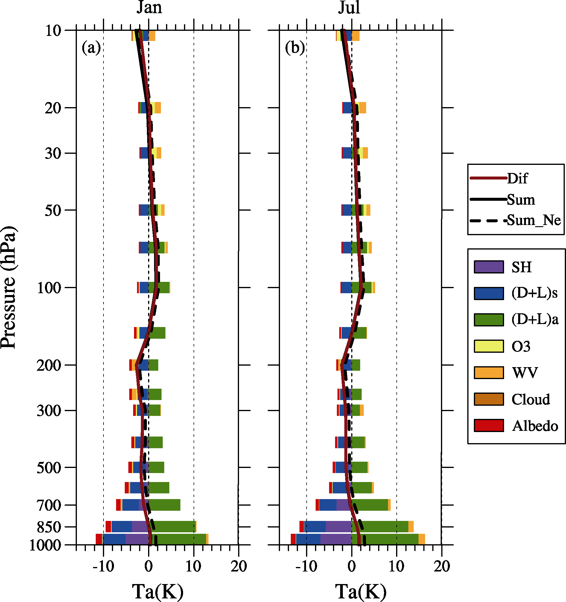
The zonal-mean Ts biases, defined as the Ts difference between FGOALS-s2 and ERA-Interim (brown curve), in January and in July are shown in Figs. 1a and 1d, respectively. It can be seen that the polar regions tend to be dominated by cold biases and the winter hemisphere is dominated by even stronger cold biases (exceeding -7 K). With regard to the colder/warmer oceanic temperature in high/low-to-middle latitudes in ERA-Interim relative to HadCRU4 (Hadley Climate Research Unit, version 4) observation data (Park et al., 2014), the model cold biases in the polar regions could be stronger compared with HadCRU4, while the model warm biases over low to middle latitudes may become smaller when compared with HadCRU4. Warm biases are found over the midlatitudes, particularly in the summer hemisphere where the maximum warm bias (~5 K) is larger than that over the tropics. To validate the decomposition by CFRAM, the sum of the partial Ts biases obtained from Eq. (5) are also shown in Figs. 1a and 1d (black solid line). It is clear that the meridional distribution, as well as the magnitude of the Ts biases, obtained through CFRAM, is almost identical to the observed Ts biases, confirming that the linearization of the radiative processes is reliable and accurate.
It should be noted that the partial temperature bias attributed to incident solar radiation at the TOA are not really model biases. It appears because the solar constant applied in FGOALS-s2 is 1365-1366 W m-2, which is recommended by CMIP5; while that applied in ERA- Interim is 1370 W m-2, which is estimated from multiple sources of data but has been known, on average, to overestimate the global solar radiation by about 2 W m-2 (Dee et al., 2011). Since the partial temperature biases by individual processes in CFRAM are capable of being added linearly, we exclude the partial temperature bias solely due to the solar difference from the total temperature bias in our attribution analysis of the model biases by other physical processes. Obviously, the meridional distribution of the Ts biases does not change significantly; only the magnitudes of warm biases become relatively larger, particularly in the low-to-middle latitudes, after the partial temperature bias due to the solar difference is excluded (black dashed line vs the black solid line in Figs. 1a and 1d).
Figure 1b presents the partial Ts biases due to individual radiative and non-radiative processes in January. Generally, compared with those due to radiative processes, the magnitudes of theTs biases due to individual non-radiative processes are remarkably lager. Specifically, larger warm biases due to the systematically overestimated downward surface sensible and latent heat fluxes are present across the winter and summer hemispheres, which are compensated for by the comparably larger cold biases due to surface dynamic processes. This suggests that, in FGOALS-s2, there may be relatively more/less energy being stored/released into the oceans/atmosphere. The magnitudes of the warm Ts biases due to atmospheric dynamics are much smaller and relatively trivial. Among the radiative processes, the cold biases due to overestimated albedo in high latitudes of the summer hemisphere are the
 | Figure 1 (a) Boreal winter (January) zonal mean Ts biases (units: K) in terms of the difference between the Flexible Global Ocean-Atmosphere- Land System model, spectral version 2 (FGOALS-s2) and the European Center for Medium-Range Weather Forecasts (ECMWF) Re-Analysis Interim (ERA-Interim) (brown solid line), the sum of all the partial Ts biases obtained from CFRAM (black solid line), and that with the partial Ts biases due to solar difference are excluded (black dashed line). (b) Zonal mean partial Ts biases due to radiative processes including ozone, water vapor, cloud, and albedo feedback, and non-radiative processes including surface sensible and latent heat fluxes, and dynamic processes at the surface and in the atmosphere in January. (c) Zonal mean partial Ts biases due to all radiative processes (red bars) and non-radiative processes (blue bars) in January (the black dashed lines in (b, c) are the same as in (a)). Panels (d-f) are similar to (a-c), but for boreal summer (July). |
strongest (up to -20 K), while the cold Ts biases in the tropics due to water vapor are related to the greenhouse effect of the underestimated water vapor content in the troposphere (Fig. 4in Yang et al., 2015). The zonal-mean Ts biases due to ozone and cloud are relatively much smaller and negligible.
The meridional distribution of the Ts biases in July is largely similar to that in January, except that the Ts biases due to surface latent heat flux in boreal summer are no longer globally positive, being negative south of 35° N with much smaller magnitudes. Accordingly, the magnitude of the cold biases due to surface dynamics is also smaller compared with that in January, suggesting smaller zonal-mean biases (or better performance) of the model in boreal summer than in boreal winter in representing the non-radiative processes that contribute to the zonal mean Ts biases.
To distinguish the relative contributions from radiative and non-radiative processes, Figs. 1c and 1f display the partial Ts biases by the two kinds of processes in January and in July, respectively. It is clear that the contributions from the radiative processes, and those from the non-radiative processes, always tend to compensate for one another, particularly over the polar region of the summer hemisphere where the cold Ts biases due to overestimated albedo are compensated for by non-radiative processes. The close compensation between radiative and non-radiative processes confirms that the coupled surface-atmosphere system always exhibits synchronized and compensatory feedbacks to energy perturbations by any physical process. Therefore, the consequent total temperature biases may not be too large, even when the model biases in representing various processes are quite large.
lists the partial Ts biases in global means. The partial Ts biases due to surface albedo, the main contributor from the radiative processes, are negative in both winter and summer, corresponding to the total radiativeTs biases of -2.38 K and -1.92 K in January and July, respectively. Consistent with the zonal-mean distribution in Fig. 1, the total warm Ts biases due to non-radiative processes (2.76 K/3.62 K in January/July) are mainly dominated by surface heat flux processes, and are partially compensated for by surface dynamic processes in both winter and summer. Due to the compensation between radiative and non-radiative biases, the overall global mean Ts biases are much smaller (0.38 K/1.70 K in January/July), despite the relatively much larger partial biases due to each of them.
| Table 1 Global-mean partial Ts biases (units: K) attributed to biases of partial radiative (Rad) processes including ozone (O3), water vapor (WV), cloud, and albedo feedback, and non-radiative (Non-rad) processes including surface sensible heat flux (SH) and latent heat flux (LH), and dynamic processes at the surface (DynS) and in the atmosphere (DynA). Note that the Ts biases attributed to the different incident solar radiation at the top of the atmosphere, which is not really model bias, are excluded when calculate the sum of Ts biases. |
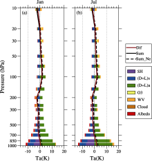
Similar to the Ts biases, we first validate that the observed global-mean Ta biases (brown curve in Fig. 2) are highly consistent with the sum of partial Ta biases obtained through CFRAM (black solid curve in Fig. 2). They both exhibit warm biases in the lower troposphere and lower stratosphere, and cold biases in the mid-to- upper troposphere and upper stratosphere, in boreal winter as well as in boreal summer. Furthermore, the total Ta biases when the partial Ta biases due to a shortage of solar radiation are excluded (black dashed line in Fig. 2), also exhibit a similar vertical distribution, albeit with the amplitudes of the warm/cold biases being slightly larger/ smaller.
Note that, unlike the effects of surface sensible heat flux on the atmosphere, which can be obtained directly, the heating rate of the surface latent heat flux in the atmospheric layer is usually unavailable in both model results and reanalysis data; the energy perturbation by surface latent heat flux (L) in CFRAM is considered as part of that by dynamical processes (D). For ease of reference, we use
 | Figure 2 Vertical profiles of the global-mean partial Ta biases (units: K) due to radiative processes and non-radiative processes (bars), the sum of all the partial Ta biases obtained from CFRAM (black solid line), that with the partial Ta biases due to solar difference excluded (black dashed line), and the Ta biases in terms of the difference between FGOALS-s2 and ERA-Interim (brown line) in (a) January and (b) July. |
It can be seen from Fig. 2 that the vertical distributions of most of the global mean partial Ta biases due to individual processes are highly similar between January and July. The magnitudes of the total Ta biases are around ± 3 K at most, while those of the individual processes are up to ± 10 K— much larger than the Ta biases we observed. This again indicates the synchronized and compensatory feedbacks to energy perturbations by any physical process within the coupled surface-atmosphere energy balance system. Specifically, the
To further quantify the relative contributions to the Ta biases, the global-mean Ta biases due to all radiative (except solar radiation) and all non-radiative processes are shown in Fig. 3. Despite the small amplitudes of the partial Ta biases by individual radiative processes, their overall contributions to the total Ta biases are comparable to those by the non-radiative processes. In the surface layer, the total warm biases (dashed line) are mainly dominated by non-radiative processes, and are compensated for by the cold biases due to radiative processes. In the mid-to-upper troposphere from 700 to 200 hPa, the radiative processes are overwhelming. In the stratosphere, biases are mostly dominated by non-radiative processes, except in the mid-stratosphere where ozone feedback largely dominates.
This study adopts an energy-balance-based decomposition
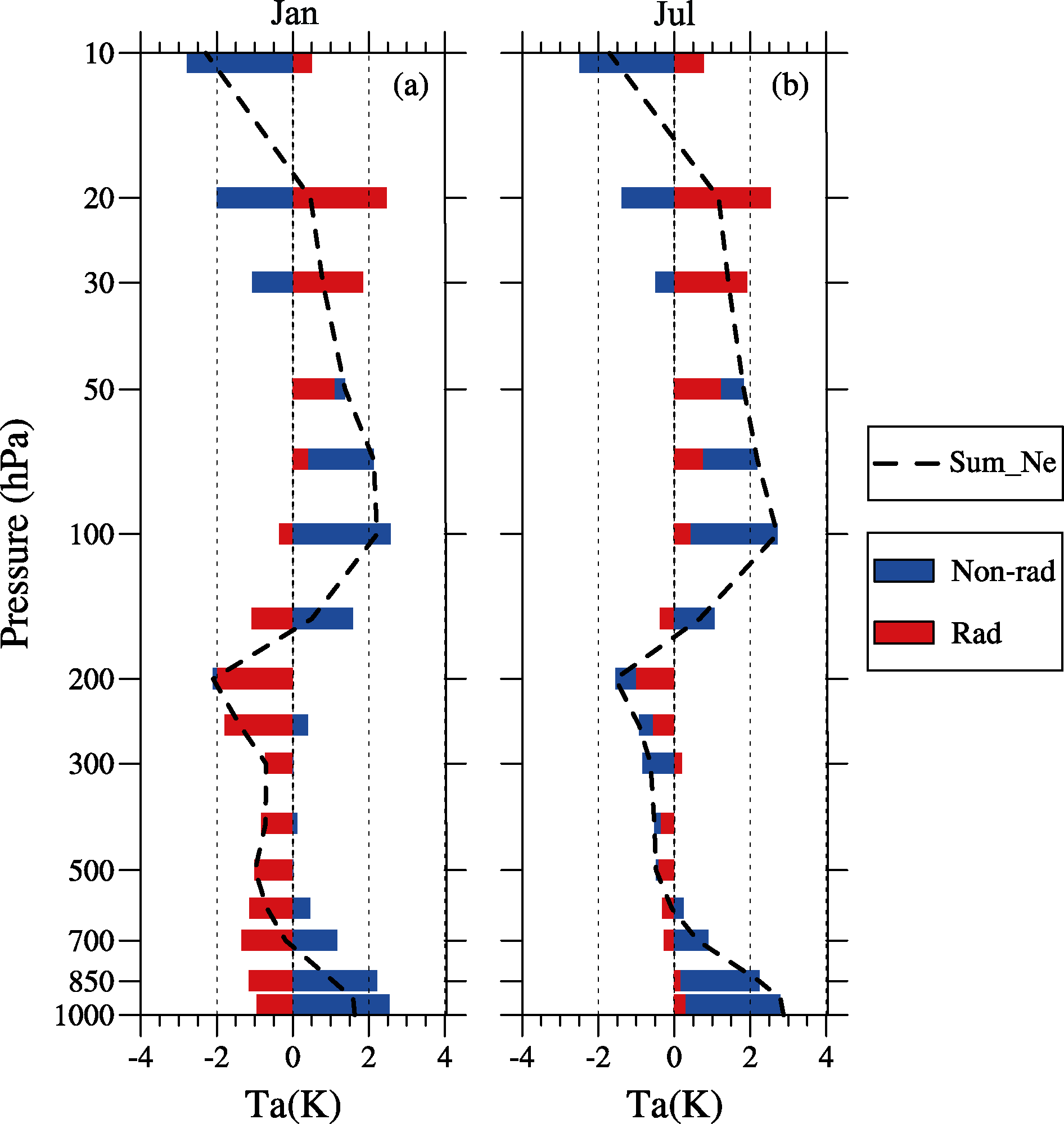 | Figure 3 Vertical profiles of the global-mean partial Ta biases (units: K) due to all the radiative processes (red bars) and non-radiative processes (blue bars), and the total model biases with the partial Ta biases due to solar differences excluded (black dashed line) in (a) January and (b) July. |
method (CFRAM), and provides a global overview of the quantitative attribution of the atmospheric and surface temperature biases in FGOALS-s2, which are defined with respect to ERA-Interim data during 1979-2005. The results show that, despite the small magnitude of the global mean Ts and Ta biases, (Ts is only 0.38 K/1.70 K in January/July, and the Ta biases from the troposphere to the stratosphere are only around ± 3 K at most), the temperature biases due to model biases in individual radiative and non-radiative processes are considerably large, with the maximums exceeding ± 10 K. Specifically, for the global-mean Ts biases, the cold biases attributed to model biases in radiative processes, mainly from albedo, act to compensate for the warm biases due to non-radiative processes, particularly the systematically overestimated downward surface heat fluxes. In terms of the vertical distribution of the global-mean Tabiases, radiative processes tend to dominate in the mid-to-upper troposphere, while non-radiative processes mainly dominate in the stratosphere, except the mid-stratosphere where the dominant contributor is the ozone feedback process.
The results of this study basically indicate that the small model temperature biases may not necessarily imply that all the physical processes in the model are represented quite well; rather, it may be the result of compensatory interactions among various processes with quite large biases. The global overview of the model biases in physical processes can also help us to understand the global features of the energy balance in the model surface-atmosphere system, and to improve the general reproducibility of the model system through improvement of the model’ s representation of related physical processes.
| 1 |
|
| 2 |
|
| 3 |
|
| 4 |
|
| 5 |
|
| 6 |
|
| 7 |
|
| 8 |
|
| 9 |
|
| 10 |
|
| 11 |
|
| 12 |
|
| 13 |
|
| 14 |
|
| 15 |
|
| 16 |
|
| 17 |
|
| 18 |
|
| 19 |
|
| 20 |
|
| 21 |
|
| 22 |
|
| 23 |
|
| 24 |
|
| 25 |
|
| 26 |
|