The statistical properties of turbulence in the urban canopy layer are of great importance due to air pollutant dispersion in the urban canopy layer, and energy and mass exchange between the atmosphere and the Earth’ s surface. However, because of the complexity of the underlying surface conditions and buildings, little is known about these properties of the urban canopy layer, unlike those in the atmospheric boundary layer (Liu and Hu, 2013; Li et al., 2014). Moreover, related studies have focused mainly on turbulent fluxes and the power spectrum (-5/3 law), whereas dissipation fields in the urban canopy layer have yet to be investigated in detail. This aspect is meaningful because the dissipation rate of turbulent kinetic energy ε is one of the key parameters of the turbulent energy cascade process, and plays an important role in turbulence parameterization schemes, such as the K-ε model and the large eddy simulation (LES) model. In order to obtain high-order moment properties of small-scale turbulent dissipation in the inertial range, the ultrasonic anemometer with a high sampling frequency of 100 Hz was used in our study.

A physical picture leading to intermittent turbulence visualizes kinetic energy flux from large scales to small scales as a self-similar cascade with an associated multiplicative process (Frisch, 1995). One of the striking signatures of the so-called intermittency phenomenon is the occurrence of non-Gaussian statistics at small scales (Hu, 1995). The energy transfer towards small scales is related to the non-zero skewness of the probability distribution function (PDF) of the velocity increments and the large flatness of the PDF (kurtosis) corresponding to the presence of strong bursts in the energy dissipation.

These intense bursts can be characterized by a singular exponent, which reflects the strength of the singularities (singular activities such as extreme events, abrupt changes) of the time series; and violent, rare events may be caused by nonlinear dynamics (Quan et al., 2007). Homogeneous signals that can be indexed by a single global singular exponent are monofractal; while nonhomogeneous multifractal signals, of which the singular exponent is a fluctuating quantity dependent on the temporal position, can be decomposed into many subsets characterized by different singular exponents quantifying the local singular behavior of the time series.

Halsey et al. (1986) introduced the singularity spectrum for the fractal dimensions of sets of singularities characterizing multifractals. The multifractal formalism has been established to account for the statistical scaling properties of singular processes and measures in many fields (Ivanov et al., 1999; Gao and Fu, 2013). The singularity spectrum has been investigated for several positive-definite quantities characterizing the small-scale motion of turbulence, especially for energy and scalar dissipation in laboratory-based turbulent flows (Meneveau and Sreenivasan, 1991; Prasad et al., 1988; Sreenivasan, 1991). Meanwhile, the singularity spectrum implies high-order moment behaviors that can also be illustrated by the scaling law of structure function of order q (Kolmogorov, 1941). With regard to the thermal dissipation in turbulent convection, Hu (1995) proposed the self-similar multiplicative cascade model providing the q-order structure function exponents, and the theory was verified via experimental observation (Hu et al., 2005) and numerical simulation based on a shell model (Song et al., 2014).

In this paper, we discuss the multifractal characteristics of energy and thermal dissipation rates in the urban canopy layer. The structure of the paper is as follows. In section 2, the experiment and data are described. In sections 3 and 4, we detect the singularity of intermittent turbulence using the wavelet transform modulus maxima method, and then investigate multifractality of the turbulent dissipation rate. A summary and conclusions are presented in section 5.

The sampling frequency of the ultrasonic anemometers used in previous atmospheric boundary layer research tended to focus approximately on the range of 10-20 Hz, which is not high enough to detect high intermittency in atmospheric turbulence. In order to obtain turbulence data with high enough temporal resolution for the wind velocity and temperature fluctuations with high intermittency (i.e., strong singularity) in the inertial range to be detected, we used the Omnidirectional and Asymmetric (R3A-100) Research Ultrasonic Anemometer in this study.

The R3A Research Anemometer is produced by Gill Instruments Ltd. in the United Kingdom and has a sampling frequency of 100 Hz. Because it can measure the sound velocity component in three directions simultaneously, while other ultrasonic anemometers can only measure the vertical component, the composed sound velocity is more accurate, and thus the wind velocity and temperature measurements are also more accurate.

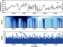
During 8-9 August 2004, an R3A Research Anemometer was installed at the 15 m level of the Beijing 325 m meteorological tower. The canopy characteristic height Laround the tower is about 50 m, enabling the turbulent flow in the urban canopy to be investigated. The weather conditions during the study period were sunny with high temperatures and low relative humidity. To discuss the intermittency of the fully developed turbulence under unstable conditions, we choose the data from about 1000 to 1200 LST (local standard time). After removing the outliers, spikes, and trends in the dataset, we examine its singularity and multifractality. A sample of the temperature fluctuations during 0958-1010 LST 9 August 2004 is presented in Fig. 1a.

The intermittency of small-scale turbulence shows the non-Gaussian behavior in the PDF of dissipation quantities increases with decreasing scale. High intermittency indicates strong singularity in the turbulent time series, which represents the cusps and steps in the data. We can see many ramp-cliff structures in the temperature fluctuations (Fig. 1a), and the singularity is strong when close to the cliff.

The Holder exponent (α ) characterizes the singularity strength of function f at the point t_i, and is defined as the largest exponent if there exists a polynomial P_n(t-t_i) of order n satisfying

, (1)

for t in the neighborhood of t_i. The polynomial P_n(t-t_i) corresponds to the Taylor expansion of faround t=t_i up to the order n and C (> 0) is a constant. Thus, the lower the exponent , the more singular the function f at the point t_i; and the higher the singular exponent, the more regular the function f.

Figure 1

	Figure Option ViewDownloadNew Window
	Figure 1 Wavelet transform modulus maxima of fully developed turbulence from turbulent convection. The analyzing wavelet is the Mexican hat wavelet. (a) The temperature time series sample during 0958-1010 LST 9 August 2004. (b) Continuous wavelet transform of the turbulent signal using the Mexican hat wavelet. (c) Wavelet transform skeleton defined by the set of all the maxima lines.

The wavelet transform has become a mathematical microscope able to reveal the singular behavior of processes and measures. Therefore, the wavelet transform can be used for singularity detection. Arneodo et al. (1995) proposed the wavelet transform modulus maxima (WTMM) method to investigate the scaling properties of singular processes (Arneodo et al., 1998; Arneodo et al., 2002), which is briefly presented here. A notable alternative is the multifractal detrended fluctuation analysis (MF-DFA) algorithm (Kantelhardt et al., 2002).

The continuous wavelet transform W of a real-valued function f is defined as

, (2)

where the function is the analyzing wavelet, b is the space parameter, and a (> 0) the scale parameter. Because the trend of the data can be represented by a polynomial, we use the analyzing wavelets defined by the second derivative of the Gaussian function— the Mexican hat wavelet in our work. Figure 1b shows the wavelet transform of the turbulent signal of which the singular behavior can be revealed.

A simple method to build the partition function Z would rely on the wavelet coefficients:

. (3)

However, nothing prevents from vanishing and the partition function would diverge for qβ < β 0. The WTMM method builds a partition function from the modulus maxima of the wavelet transform. The maxima are defined as the local maxima of considered as a function of x at each scale a. As illustrated in Fig. 1c, these WTMM are deployed on connected curves called maxima lines. Let L(a₀) be the set of all the maxima lines that exist at the scale a₀ and which contain maxima at any scale aβ ≤ β a₀. In the case of a fractal signal, we expect the number of maxima lines to converge in the limit a→ 0. The skeleton of the wavelet transform is created by all of its maxima lines. The WTMM skeleton reveals the hierarchical organization of the singularities, so the partition function will be defined by this skeleton and by summing up the qth power of these maxima:

, (4)

Where the ‘ sup’ defines a scale-adaptive partition that prevents divergences.

The WTMM method changes the continuous sum over

space into a discrete sum over the local maxima of

. The method reveals the scaling structure of

the singularities, and that it is scale-adaptive.

Intermittent distributions for several quantities characterizing small-scale motion in fully developed turbulence can be described in terms of singularities of varying strength, which lie on sets of different fractal dimensions, and are called multifractal. So, in this section, we investigate the multifractality of the most important quantity— the turbulent dissipation rate.

The dissipation rate of turbulent kinetic energy is defined by , whereu is the longitude velocity fluctuation and denotes kinematic viscosity. Another quantity of practical interest is the thermal dissipation rate , where x_i represent the spatial coordinate, T is the temperature fluctuation, and is the thermal diffusivity of the fluid. Because the flows have a mean velocity that is high compared with turbulent fluctuations, we use Taylor’ s frozen-flow hypothesis to simplify the calculation of the dissipation rate by , where denotes the mean velocity. Hence, the energy and thermal dissipation rates can be represented by and , respectively, and are calculated using simple finite differences. We analyze the normalized energy dissipation rate and the thermal dissipation rate for convenience. Here, < > means the statistical average.

Scaling behavior is often observed for the partition functionZ(q, a), and scaling exponents τ (q) can be defined that describe how Z (q, a) scales with a:

. (5)

The mass exponents, τ (q), characterize the multifractal properties of the series under investigation. Because the singularity spectrum f(α ) can be determined by the Legendre transform of τ (q), the singular exponents α can be calculated by

. (6)

The generalized fractal dimensions D(q), which correspond to the scaling exponents for the qth moments of the singular measure, are obtained by the following relation:

. (7)

By analyzing the wavelet transform scaling behavior along the maxima lines, the value of the singular exponents α can be estimated according to

, (8)

and theoretically, the exponents are identical to those in

Eq. (6). The singularity spectrum f(α ) is defined as the

Hausdorff dimension of the set of all points x such that

, which can be determined by

. (9)

Therefore, the statistical properties of the different subsets characterized by these different exponents can be quantified by the function f(α ), where f(α ₀) denotes the fractal dimension of the subset of the time series characterized by the singular exponent α ₀. Monofractal time series can be characterized by the roughness exponent called the Hurst exponent H; while for multifractal time series, the generalized Hurst exponent H(q), which is dependent of q, could be used. We can obtain H(q) by the following equation:

. (10)

The data were separated into 12 segments, each of which was 10 min long, and obtained the resulting values by averaging all the results of the samples. For nonhomogeneous processes, positive moments q enhanced the spiky regions and strong singularities, whereas negative q emphasized the smooth regions and weak singularities. No convincing scaling was observed for qβ < β 0 in our study; and since the uncertainty in the determination of for qβ < β 0 is relatively high, only the results for qβ ≥ β 0 are calculated.

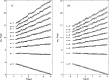
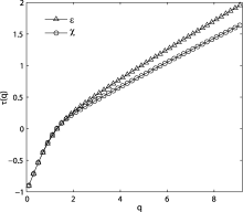
Figure 2 shows the partition functions Z(q, a) of the energy dissipation rate ε and thermal dissipation rate χ performed with the WTMM method. The analysis is limited within the range of qβ =β [0, 9] and the scale a is in the region 20β < β aβ < β 500. For the broad range of q, the partition function Z(q, a) scales with scales a as a power law. When q is smaller than 3, the correlation coefficient of the least square fitting is larger than 0.97. Even the smallest correlation coefficient is 0.92 (when qβ =β 9). The mass exponents τ (q) of the two kinds of dissipation rate are obtained from the slope of the partition function curves, which are shown in Fig. 3. Monofractal signals display a linear τ (q) spectrum. On the contrary, a nonlinear τ (q) curve is a signature of nonhomogeneous processes that displays multifractal properties, in the sense that the singular exponent is a fluctuating quantity that depends upon the temporal position. As shown in Fig. 3, when plotted versus q, the mass scaling exponents τ (q) obtained for the experimental turbulent signal deviate distinctly from a straight line. The mass exponents for the temperature field have slightly stronger nonlinearity than those for the velocity field, especially for high moments.

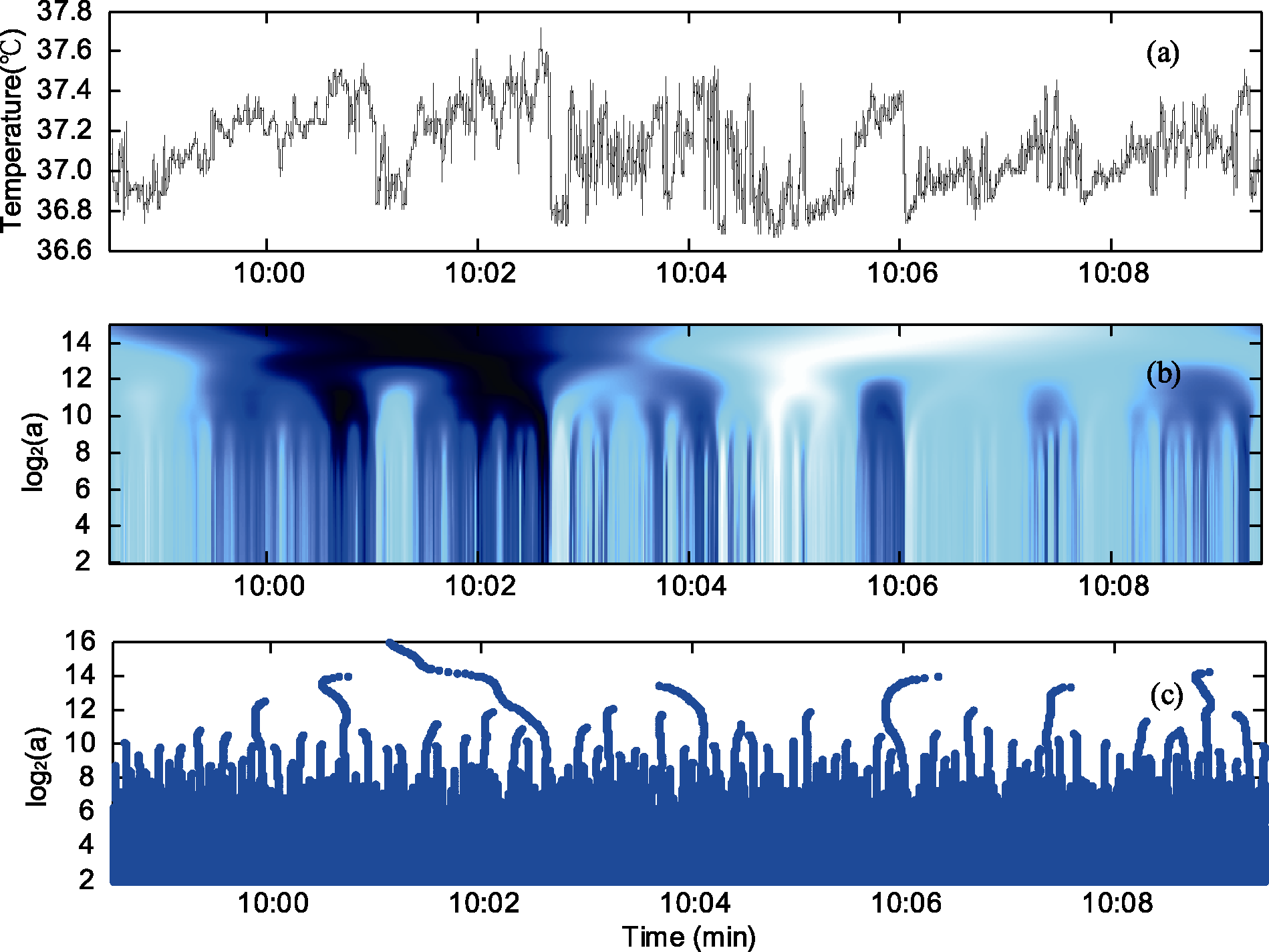
The corresponding f(α ) singularity spectrum for the energy and thermal dissipation rates obtained by Legendre transforming τ (q) are shown in Fig. 4. Its characteristic concave function shape over the range of singular exponents is a clear signature of the multifractality of the turbulent dissipation field. For the monofractal signal, the singularity spectrum is a single point. For χ , the values of α when varying q from 0 to 9 range in the interval [0.18, 0.93]. The minimum α corresponds to the largest singularity in the distribution, and the maximum α corresponds to its least intense regions. For qβ =β 0, the largest dimension is attained for singularities of exponent , and the corresponding maximum of thef(α ) curve, does not deviate from D_Hβ =β 1. Together with the upper bound , this suggests that the turbulent signal could be singular everywhere. Moreover, the dimension of the set of all singularities of the thermal dissipation is definitely less than 1. The singular exponents are most frequently encountered around 0.2 for the temperature field, which are significantly smaller than the theoretical value of , predicted by Kolmogorov (1941). Also, the most frequent singular exponents are smaller than those for a wind tunnel at a moderate Reynolds number (Arneodo et al., 1998). The

Figure 2

	Figure Option ViewDownloadNew Window
	Figure 2 The partition function Z(q, a) of the (a) energy dissipation rate ε and (b) thermal dissipation rate χ in a log-log plot performed using the WTMM method. The analysis is limited within the range of qβ =β [0, 9]. The same analyzing wavelet as in Fig. 1 is used.

Figure 3

	Figure Option ViewDownloadNew Window
	Figure 3 The q-order mass exponents τ (q) of the energy dissipation rate ε and thermal dissipation rate χ .

Figure 4

	Figure Option ViewDownloadNew Window
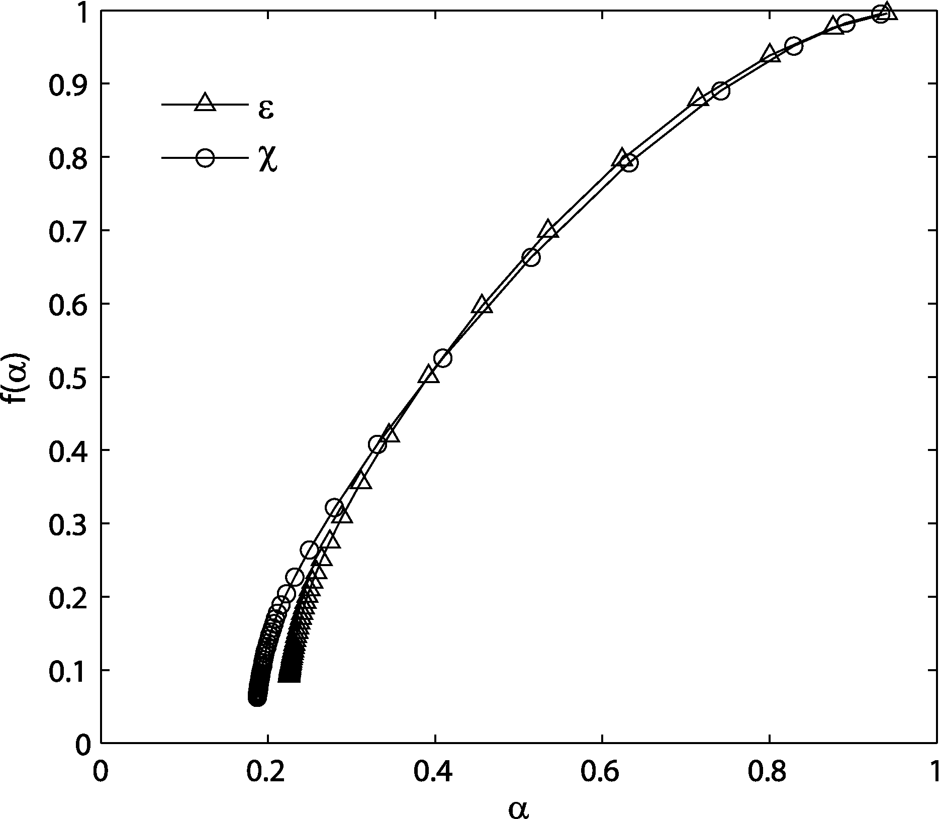	Figure 4 The singularity spectrum f(α ) curve of the energy dissipation rate ε and thermal dissipation rate χ .

evidence indicates a higher intermittency of turbulence in the atmospheric surface layer at a high Reynolds number, which is revealed by the data with high temporal resolution. Similar results can be obtained for ε . However, there are slight differences between the singularity spectrum for ε and χ . From Fig. 4, it can be seen that for χ , which is lower than observed for ε ( ). This means that χ has stronger singularities than ε . The parameter spectrum width , which is defined by the range of singular exponents and reflects the strength of the multifractal behavior, is 0.75 for χ , and it is larger than 0.71 for ε . This is the signature that the temperature field is more intermittent than the velocity field: the f(α ) singularity spectrum for the former is slightly wider than the corresponding spectrum for the latter. Also, the intermittency exponent is given in terms of the curve as , evaluated at qβ =β 0. We can obtain , higher than the intermittency exponent of ε ( ).

The generalized Hurst exponents H(q) of the energy dissipation rate ε and thermal dissipation rate χ are given in Fig. 5. For positive values of q, H(q) describes the scaling behavior of large fluctuations. Usually, the large fluctuations are characterized by a smaller scaling exponent H(q) for multifractal series, meaning weaker long-range correlation. So, the long-range correlation for the velocity field is stronger than that for the temperature field at high-order moments.

Figure 5

	Figure Option ViewDownloadNew Window
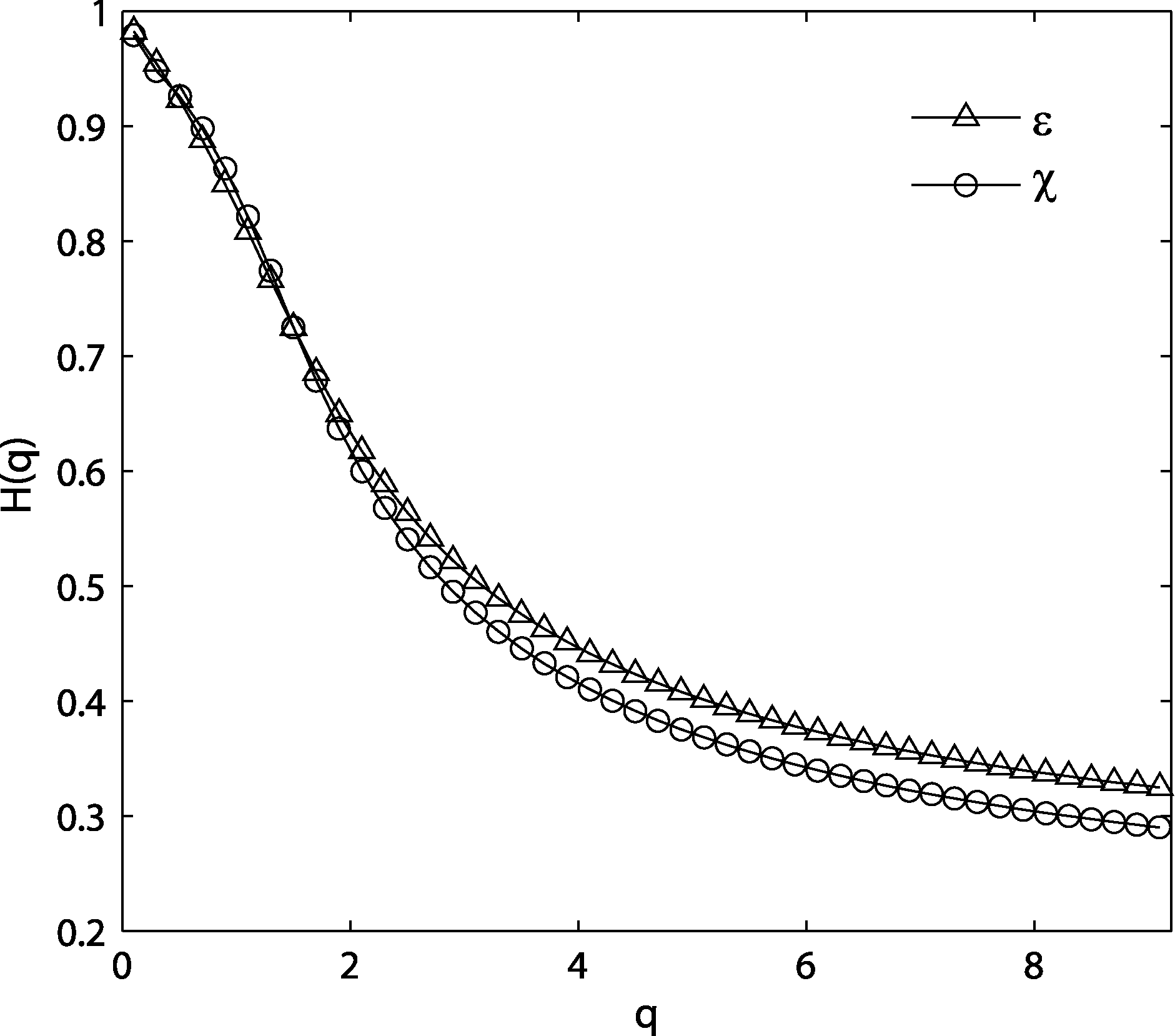	Figure 5 The generalized Hurst exponents H(q) of the energy dissipation rate ε and thermal dissipation rate χ .

In this paper, we investigate the multifractality of the dissipation field of small-scale intermittent turbulence in the urban canopy layer by a useful characterization of intermittency— the singularity spectrum f(α ). The observation that the dissipation field has a multifractal distribution supports the notion of a self-similar multiplicative process occurring in turbulent flows. The main conclusions are summarized as follows.

The parabola shape of the singularity spectrum f(α ) over the range of singular exponents indicates the multifractality of the turbulent dissipation field; and the singular exponents being smaller than 1 implies that the turbulent signal could be singular everywhere. Moreover, the singular exponents of the energy and thermal dissipation rates are most frequently encountered at around 0.2, which is significantly smaller than the theoretical value of predicted by Kolmogorov (1941) and the singular exponents for a wind tunnel at a moderate Reynolds number. The evidence indicates a higher intermittency of turbulence in the urban canopy layer at a high Reynolds number, which is revealed by the data with high sampling frequency. Furthermore, the fact that the minimum singular exponent for thermal dissipation is lower than that for energy dissipation, that the singularity spectrum for the former is slightly wider than the corresponding spectrum for the latter, and that the intermittency exponent μ of the thermal dissipation rate is higher, means that the temperature field is more intermittent than the velocity field. The above result is also demonstrated by the evidence that the mass exponent curve for the temperature field has slightly stronger nonlinearity than for the velocity field, especially on high-order moments, and the long-range correlation of thermal dissipation characterized by smaller Hurst exponents is weaker than that of energy dissipation on high-order moments.

Due to the large integral scale of turbulence in the atmospheric boundary layer and experimental uncertainty about high-order moments, the tail of the singularity spectrum curve for the atmosphere is very hard to obtain with absolute accuracy. So, a large amount of samples could be used for verification of the results. Meanwhile, the degree of correlation existing among joint distributions of intermittent quantities in turbulence, such as the dissipation of kinetic energy and the dissipation of passive scalar fluctuations, can be described well by extending the multifractal formalism to more than one variable.