Different Warming Patterns of Tropical Pacific Sea Surface Temperature Projected by FGOALS-g2 and FGOALS-s2 under RCP8.5
[ZHANG Li-Xia1, 2  , ZHOU Tian-Jun
1, 3 ]
, ZHOU Tian-Jun|
|


Citation: Zhang, L.-X., and T.-J. Zhou, 2015: Different warming patterns of tropical Pacific sea surface temperature projected by FGOALS-g2 and FGOALS-s2 under RCP8.5, Atmos. Oceanic Sci. Lett., 8, 82-87.
doi:10.3878/APSL20140070.
Received:20 August 2014; revised:6 February 2015; accepted:10 February 2015; published:16 March 2015
The different patterns of SST changes under the +8.5 W m-2 Representative Concentration Pathway (RCP8.5) projected by the latest two versions of the Flexible Global Ocean-Atmosphere-Land System model (FGOALS-g2 and FGOALS-s2; grid-point version 2 and spectral version 2, respectively), and the potential mechanisms for their formation are studied in this paper. The results show that, although both FGOALS-g2 and FGOALS-s2 project global warming patterns, FGOALS-g2 (FGOALS-s2) projects a La Niña-like (an El Niño-like) mean warming pattern with weakest (strongest) warming over the central (eastern) equatorial Pacific for 2081-2100 relative to 1986-2005 under RCP8.5. A mixed layer heat budget analysis shows that the projected tropical Pacific Ocean warming in both models is primarily caused by atmospheric forcing. The main differences in the heating terms contributing to the SST changes between the two models are seen in the downward longwave radiation and ocean forcing. The minimum SST warming over the equatorial Pacific in FGOALS-g2 is attributed to the local minimum heating of downward longwave radiation and maximum cooling of ocean forcing. In contrast, the maximum SST warming over the equatorial Pacific in FGOALS-s2 is due to the maximum warming of downward longwave radiation, and the contribution of ocean forcing is minor. The minimum SST warming over the equatorial Pacific in FGOALS-g2 emerges around the 2050s, before when the SST over the equatorial Pacific is warmer than that over the extra-equatorial Pacific. In FGOALS-s2, the SST difference shows a continuous increasing trend for 2006- 2100. Further examination of the oceanic and atmospheric circulation changes is needed to reveal the process responsible for the longwave radiation and ocean forcing difference between the two models.
The ocean plays an important role in the climate system due to its large heat capacity. In recent decades, a warming trend has been observed in the global ocean (Bindoff et al., 2007). Although the warming magnitude of the ocean is much smaller than that of land, small changes in tropical SST can exert a great impact on global climate, such as the El Niñ o-Southern Oscillation (ENSO) and basin-wide warming of the Indian Ocean (Lau and Weng, 1999; Hoerling et al., 2004; Du and Xie, 2008; Dong and Zhou, 2014). Tropical precipitation changes are positively correlated with spatial deviations of SST warming from the tropical mean (Xie et al., 2010). Thus, it is important to study how SST might change in the future.
Previous studies have investigated the response of SST changes to global warming. Many studies document that the increasing concentrations of carbon dioxide (CO2) and other greenhouse gases (GHGs) in the atmosphere are considered as the major sources for ocean warming (Meehl et al., 2007). For example, the basin-wide warming trend of the Indian Ocean SST since the 1950s is largely attributed to external forcing, and 98.8% of the contribution is from anthropogenic forcing (Dong and Zhou, 2014). However, based upon the results of climate models, agreement on the response of SST over the Pacific Ocean to increased GHGs has not yet been reached. Using the Cane-Zebiak model, a La Niñ a-like state is predicted in response to warming, in which the ocean thermostat mechanism dominates (Clement et al., 2006). The mixed-layer global climate models (GCMs) in 13 models from phase 3 of the Coupled Model Intercomparison Project (CMIP3) database show El Niñ o-like warming patterns in response to a CO2 doubling, due to weakened Walker circulation over the tropical Pacific; while a slightly larger warming in the central Pacific than the western Pacific, or “ El Niñ o-ness” warming, is seen in the fully coupled GCMs (Vecchi et al., 2008). Vecchi et al. (2008) suggest that the reduced response in free coupled GCMs relative to mixed-layer models results from a superposition of both the ocean thermostat and the weaker Walker mechanisms. The CMIP3 model projections show different responses of their ENSO variability to global warming (Merryfield, 2006). For the Representative Concentration Pathways (RCPs) with new models in phase 5 of CMIP (CMIP5), a discrepancy in the responses of SST to global warming still exists (Collins et al., 2014).
To date, the tropical Pacific Walker circulation (Ma and Zhou, 2014), the interannual variability modes of the East Asian summer monsoon and western North Pacific subtropical high (He and Zhou, 2014; Song and Zhou, 2014), monsoon (Bao, 2012; Zhang and Zhou, 2014), and projected drought under the +8.5 W m-2RCP scenario (RCP8.5) (Zhou and Hong, 2013) have been examined in many studies. Considering the importance of SST warming patterns to global climate, it is desirable to assess the SST patterns in a potentially warmer future climate. The main motivation of the present study is to examine the differences in the SST changes under RCP8.5 (Moss et al., 2010) between the outputs of the two latest versions of the Flexible Global Ocean-Atmosphere-Land System model (FGOALS-g2 and FGOALS-s2; grid-point version g2 and spectral version 2, respectively), developed at the State Key Laboratory of Numerical Modeling for Atmospheric Sciences and Geophysical Fluid Dynamics (LASG), Institute of Atmospheric Physics (IAP).
The reminder of the paper is organized as follows: In section 2, we describe the model data and analysis method. Section 3 presents the different projected SST changes and the potential mechanisms in FGOALS-g2 and FGOALS-s2. Finally, a summary and discussion is presented in section 4.
The datasets used in this study are the historical simulations and projections under RCP8.5 simulated by the two models, i.e. FGOALS-g2 and FGOALS-s2 (see Li et al. (2013) and Bao et al. (2012) for more details of the models). The historical simulations are performed with various combinations of forcings, including GHGs, sulfate aerosols, ozone, volcanic aerosols, and solar variability. A full list of the forcing data for the historical runs of these two models can be found in Zhou et al. (2013). The RCPs include the time paths for concentrations of the full suite of greenhouse gases, aerosols, and chemically active gases.
To analyze the pattern formation of SST change, a mixed-layer heat budget analysis, following Xie et al. (2010) and Dong and Zhou (2014), is employed. For the slowly increasing GHGs scenario, SST tendency is one order smaller than the changes of net surface heat flux and ocean heat transport. The pattern formation of SST change (T′ ) can be obtained by the equation
where T′ is SST change, and
where
Based on this assumption, a simple theoretical model was constructed by Zhang and Li (2014) to reveal the cause of future patterns of SST warming. In this model, the changes of SST (T′ ) can be diagnosed by transforming the equation into
where T and V are the present-day climatological mean SST and surface wind speed, respectively; γ is a coefficient for calculating future change of sensible heat; ρ is the air density near the surface; CH is the heat exchange coefficient of SH′ ; Cp is the specific heat capacity at constant pressure, σ is the Stefan-Boltzmann constant, or Stefan's constant; and
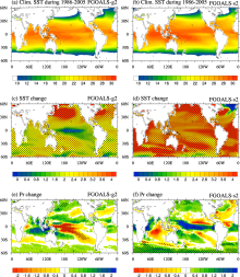
Before examining the projected SST changes, the simulated climatological SST patterns for the present day are firstly evaluated (Figs. 1a and 1b). The observed geographical distribution of SST can be simulated well by the two models, including the cold tongue over the eastern tropical Pacific and warm pool over the western Pacific Ocean and eastern Indian Ocean. The pattern correlation coefficients of the simulated SSTs by the two models with respect to the observation are both higher than 0.9. The projected SST changes for the 2081-2100 mean relative to the reference period of 1986-2005 simulated by FGOALS-g2 and FGOALS-s2 are shown in Figs. 1c and 1d. Both FGOALS-g2 and FGOALS-s2 project global warming SST changes under RCP8.5, with stronger magnitude in FGOALS-s2. However, the SST warming is not uniform everywhere. FGOALS-g2 (Fig. 1c) projects a La Niñ a-like warming pattern. The largest warming is greater than 4° C, located in the North Pacific Ocean; while the weakest warming is seen over the central equatorial Pacific Ocean, with the smallest magnitude being about 0° C. In contrast, an El Niñ o-like warming pattern is projected by FGOALS-s2 (Fig. 1d), which projects the greatest warming over the eastern equatorial Pacific Ocean, with the magnitude larger than 4° C. Associated with the different projected SST changes, the precipitation changes show opposite changes in the two models. In FGOALS- g2 (Fig. 1e), there is less rainfall in the tropical Pacific Ocean (central value of less than -2 mm d-1), while there is excessive rainfall over the tropical Indian Ocean (central value of greater than 2 mm d-1). The opposite precipitation change is projected by FGOALS-s2 and the strength is comparable with that projected by FGOALS- g2 (Figs. 1e and 1f).
 | Figure 1 Geopotential distribution of the climatological annual mean SST (units: ° C) in (a) Flexible Global Ocean-Atmosphere-Land System model grid-point version 2 (FGOALS-g2) and (b) spectral version 2 (FGOALS-s2) for 1986-2005. Panels (c, d) are the same as (a, b), but for the projected SST changes in 2081-2100 with respect to 1986-2005 under the + 8.5 W m-2 Representative Concentration Pathway (RCP8.5). Panels (e, f) are the same as (c, d), but for projected precipitation changes (units: mm d-1). The dotted areas in (c, f) are statistically significant at 0.05 level. |
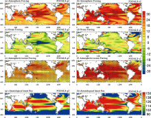
To investigate the mechanisms responsible for the different SST warming patterns projected by FGOALS-g2 and FGOALS-s2, a mixed-layer heat budget analysis is performed and reported in this section. According to Eq. (1), the changes in atmospheric forcing via radiative and turbulence fluxes (Qa′ ), ocean heat transport effect (Do′ ) and their combined effect are shown in Fig. 2. In FGOALS-g2, Qa′ heats the whole tropical ocean with the maximum and significant warming located in the central equatorial Pacific Ocean, exceeding 30 W m-2 (Fig. 2a). The ocean heat transport effect shows opposite heating anomalies to the atmospheric forcing (Fig. 2c). For the combined effect (Fig. 2e), the weakest warming effect is seen over the central equatorial Pacific, with a similar pattern to the SST warming pattern in FGOALS-g2. In FGOALS-s2, the significant atmospheric forcing is mostly seen over the tropical ocean (Fig. 2b), while the warming over the eastern tropical Pacific is not statistically significant. We can see the heating effect of the ocean forcing is statistically insignificant over all tropical oceans, with a slight warming in the tropical central Pacific Ocean (5° S-5° N, 150° E-170° W) (Fig. 2d). The difference between the two models in the projected net heating of the atmosphere and ocean forcings should be noted. The weakest warming is seen over the central tropical Pacific in FGOALS-g2, while it is over the eastern tropical Pacific in FGOALS-s2. We know that the SST formation pattern is determined not only by the net heating but also by the climatological mean latent heat flux (Eq. (1)). For the present-day, the climatological latent heat fluxes (
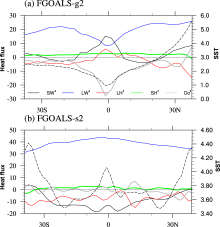
To examine which part of the atmospheric forcing contributes to the SST change patterns, the zonal mean SST and the contributions from each of the five terms in Eq. (3) over the Pacific Ocean are shown in Fig. 3. The dotted black lines in Figs. 3a and 3b are the SST changes obtained from the two models. A minimum/maximum SST warming change is seen over the equator (5° S-5° N) relative to the extra-equator (30-5° S and 5-30° N) regions in FGOALS-g2/FGOALS-s2, which is consistent with the SST change patterns shown in Figs. 1c and 1d. Both in FGOALS-g2 and FGOALS-s2, among all the atmospheric forcing terms, the largest heating changes are from the downward longwave radiation changes (LW′ , blue line). The changes in sensible heat (SH′ , green line) are generally small over the whole Pacific Ocean projected by both models. In FGOALS-g2 (Fig. 3a), consistent with the minimum SST warming over the equatorial Pacific, the minimum longwave radiation heating (LW′ ) and maximum cooling of ocean forcing (Do′ , grey line) changes are seen over the equatorial Pacific, while the maximum heating of shortwave radiation (SW′ , black line) and latent heat flux (LH′ , red line) changes in the equatorial Pacific are opposite to the SST change. This indicates that the SW’ and LH’ are the consequences of SST changes, because the weaker SST warming over the equatorial Pacific will depress local convection, leading to less cloud and deficient precipitation, and thus more SW absorption and less LH release (more LH′ , as shown in Fig. 3a). In FGOALS-s2 (Fig. 3b), a peak LW′ dominates the equatorial Pacific, while Do′ and SH′ are both small, and the SW′ and LH′ act to damp the heating effect of LW′ . By comparing the forcings projected by FGOALS-g2 and FGOALS-s2, the weaker SST warming over the tropical Pacific projected by FGOALS-g2 is mostly due to the effect of maximum ocean cooling and minimum warming of longwave radiation heating over the tropical central Pacific Ocean, while the stronger SST warming over the equatorial Pacific projected by FGOALS-s2 is mainly the result of the more substantial downward longwave radiation there.
 | Figure 2 The changes of (a, b) atmospheric forcing via radiative and turbulent fluxes ( |
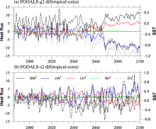
To examine the evolution of the SST warming pattern over the Pacific, the projected changes of SST difference between the equatorial Pacific (5° S-5° N) and extra-equatorial Pacific (20-10° S, 10-20° N) and the corresponding heat changes are shown in Fig. 4. The projected SST difference between the equator and extra-equator by FGOALS-g2, as discussed above, is not always less than zero for 2006-2100. It is above zero for 2006-2050, but cools after the 2050s and persists until 2100 (Fig. 4a). Accompanied by the SST changes, the longwave radiation and ocean forcings show consistent changes with the SST difference, while latent heat flux and shortwave radiation show opposite signs to the SST difference (Fig. 4a). This means that, along with the changes in the concentrations of the full suite of GHGs, aerosols, and chemically active gases under RCP8.5, the response of longwave radiation and ocean forcing over the equatorial Pacific is to change sign around the 2050s, contributing to the SST warming pattern changes. In contrast, the SST difference in FGOALS-s2 shows a continuous increasing trend from 2006 to 2100, which is mainly induced by the increased longwave radiation (Fig. 4b).
 | Figure 3 Zonal mean changes of SST (T′ , right axis, dashed black line, units: ° C) and the five terms (left axis, units: W m-2) in the numerators of Eq. (3) contributing to SST changes, including net shortwave radiation (SW′ , black lines), downward longwave radiation (LW′ , blue lines), latent heat flux (LH′ , red lines), sensible heat flux (SH′ , green lines), and ocean forcing (Do′ , grey lines) over the Pacific (180° E-60° W) derived from (a) FGOALS-g2 and (b) FGOALS-s2. |
The projected SST changes under RCP8.5 by the two latest versions of FGOALS (FGOALS-g2 and FGOALS-s2) and their formation mechanisms are examined in this paper. The results show that, although both models project global warming, FGOALS-g2 and FGOALS-s2 project different mean SST change patterns for 2081-2100 relative to 1986-2005 under RCP8.5. A La Niñ a-like warming pattern is projected by FGOALS-g2, with the smallest warming over the equatorial central Pacific Ocean; while an El Niñ o-like warming is seen in FGOALS-s2, with the greatest warming over the central equatorial Pacific Ocean. Through a mixed-layer heat budget analysis and a simple heat budget model analysis, it is found that the tropical ocean warming in both models is primarily caused by atmospheric forcing via radiative and turbulent fluxes. The minimum SST warming over the equatorial Pacific relative to the extra-equatorial Pacific in FGOALS-g2 is attributed to the minimum heating of downward longwave radiation and maximum cooling of ocean forcing. In contrast, the maximum SST warming over the equatorial Pacific projected by FGOALS-s2 is due to the maximum warming of downward longwave radiation, which is damped by shortwave radiation and latent heat flux, and the contribution of ocean forcing is minor. Examination of the evolution of the SST difference between the equatorial Pacific and extra-equatorial Pacific shows that the minimum SST warming over the equatorial Pacific in FGOALS-g2 emerges around the 2050s, before when the SST over the equatorial Pacific is warmer than that over the extra-equatorial Pacific, which is also associated with the same evolution of downward longwave radiation and ocean forcing. In FGOALS-s2, the SST difference shows a continuous increasing trend for 2006- 2100, which is mainly induced by the increased longwave radiation.
 | Figure 4 The time series for the SST difference anomalies (right axis, dashed black line, units: ° C) and the five anomaly terms (left axis, units: W m-2) in the numerators of Eq. (3) contributing to SST changes between the equatorial Pacific (5° S-5° N, 180° E-60° W) and extra-equatorial Pacific (average mean of (20-10° S, 180° E-60° W) and (10-20° N, 180° E-60° W)): (a) FGOALS-g2; (b) FGOALS-s2. |
Although based on Eq. (3), the future change in SST is determined by the changes in net solar radiation, downward longwave radiation, surface latent and sensible heat flux, and oceanic forcings. In other words, the SST change is a result of complex air-sea interaction. The downward longwave radiation changes result not only from the change in GHGs, but also from changes in cloud, air temperature and moisture. As Zhang and Li (2014) pointed out, this simple model represents a surface heat balance between uniform incoming longwave radiative forcing due to GHGs and outgoing longwave radiation and latent heat flux from the surface. This surface heat balance change is a result of the combination of atmospheric and oceanic circulation changes. We still cannot determine what physical processes contribute to the different distributions of longwave radiation and oceanic forcing changes in FGOALS-g2 and FGOALS-s2. Furthermore, what causes the abrupt changes in SST difference between the equatorial Pacific and extra-equatorial Pacific in FGOALS-g2 around 2050 remains unclear. Is it a decadal variation of the climate system, or is it due to processes changing at around that time in FGOALS-g2? Therefore, further examination of the oceanic and atmospheric circulation changes are needed.
| 1 |
|
| 2 |
|
| 3 |
|
| 4 |
|
| 5 |
|
| 6 |
|
| 7 |
|
| 8 |
|
| 9 |
|
| 10 |
|
| 11 |
|
| 12 |
|
| 13 |
|
| 14 |
|
| 15 |
|
| 16 |
|
| 17 |
|
| 18 |
|
| 19 |
|
| 20 |
|
| 21 |
|
| 22 |
|