
Simulated Heat Sink in the Southern Ocean and Its Contribution to the Recent Hiatus Decade
[OU Nian-Sen1, 4 , LIN Yi-Hua2, 1, *  , BI Xun-Qiang
3 ]
, BI Xun-Qiang|
|


Citation: Ou N.-S., Y.-H Lin, and X.-Q. Bi, 2015: Simulated heat sink in the Southern Ocean and its contribution to the recent hiatus decade, Atmos. Oceanic Sci. Lett., 8, 174-178.
doi:10.3878/AOSL20150008.
Received 10 January 2015; revised 13 February 2015; accepted 16 February 2015; published 16 May 2015A set of numerical experiments is designed and carried out to understand a heat sink in the Southern Ocean in the recent hiatus decade. By using an oceanic general circulation model, the authors focus on the contributions from two types of forcing: wind stress and thermohaline forcing. The simulated results show that the heat sink in the upper Southern Ocean comes mainly from thermohaline forcing; while in the deeper layers, wind stress forcing also plays an important role. These different contributions may be due to different physical processes for the heat budget. The combination of these two types of forcing shows a significant heat sink in the Southern Ocean in the recent hiatus decade, and this is consistent with the observations and conclusions of a similar recently published study.
Despite the anthropogenic greenhouse gas forcing is increasing, the linear trend of global mean surface temperature after 1998 is almost zero according to the Fifth Assessment Report of the Intergovernmental Panel on Climate Change (IPCC, 2013). Thus, the last decade has become known as a hiatus decade (Meehl et al., 2011). As shown by Llovel et al. (2014), ocean warming above 2000 m explains 32% of the global mean sea-level rise observed from satellite altimetry. The heat is believed to still be building up somewhere in the climate system over the recent hiatus decade, but scientists have not arrived at a consensus as precisely where, hence the term “ missing heat” (Tollefson, 2014). Previous studies show that this missing heat could be transported to deeper ocean depths (e.g., Meehl et al., 2011; Meehl and Hu, 2013; Yu and Song, 2013; Song et al., 2014). Chen and Tung (2014) further show that the hiatus decade could be caused mainly by heat transported to intermediate depths of the Atlantic and Southern oceans. They suggested a heat sink in the deeper Atlantic is initiated by a salinity anomaly in the subpolar region. However, the mechanism for the heat sink in the Southern Ocean remains unclear. Durack et al. (2014) further showed that poor sampling of the Southern Hemisphere contributes to the low bias of the global upper heat content change. Thus, additional examination of the heat change in the Southern Ocean is worthy of attention.
The Southern Ocean is the only oceanic domain that completely encircles the globe. It connects the Pacific, Atlantic, and Indian oceans, and can transmit climatic signals among them (Gille, 2002). Thus, it plays a critical role in global climate change. One important feature of the Southern Ocean is that deep convection occurs over a large domain. Due to this deep convection, the heat exchange between the water mass and the overlaying atmosphere is fast and effective, and can extend to 2 km deep (Nowlin and Klinck, 1986). Under a global-warming climate, a warming of the Southern Ocean has been revealed by observations and climate models (e.g., Gille, 2002; Song et al., 2014). Another feature of the oceanic circulation in the Southern Ocean is the prevailing ocean surface westerly, which forms a full circle around the Antarctic. Wind stress is the main forcing in maintaining the large-scale oceanic circulation in the Southern Ocean, especially the Antarctic Circumpolar Circulation (England, 1993).
Since the heat exchange between the water mass and the atmosphere in the Southern Ocean can occur directly through deep convection, and happen indirectly via wind through Ekman pumping, we are motivated to examine the combined and individual contributions of wind stress and thermohaline forcing. Observations for the Southern Ocean are sparse in both spatial and temporal terms, even sparser at intermediate depths, and almost none at depth deeper than 1500 m (Gille, 2002). In addition, it is difficult to separate the effects of wind stress and thermohaline forcing based on observed data. Accordingly, we use an oceanic general circulation model (OGCM) to simulate the heat sink in the Southern Ocean and examine the different contributions from these two types of forcing.
The OGCM used in this study is the Pressure Coordinate Ocean Model (PCOM). PCOM was originally developed by Huang et al. (2001), and further developed and applied by Zhang (2013) to study the energy balance in the world ocean. The model is constructed from 60 pressure-η levels, corresponding to approximately 15 m at the top and about 250 m in the bottom layer in a z-coordinate model. The horizontal resolution is a 1° × 1° rectangular grid. Note that for vertical mixing, instead of using a mixing scheme, we adopted a climatic dataset of turbulent mixing calculated by Zhang et al. (2014), based on real energy sources. The atmospheric forcing consists of seven variables: zonal and meridional wind stress (ZWS and MWS), sea level pressure (SLP), observed sea surface temperature (OSST), observed sea surface salinity (OSSS), fresh water flux (evaporation minus precipitation, EMP), and net downward heat flux (DHF). The simulated sea surface temperature (SST) and sea surface salinity are damped back to OSST and OSSS, respectively, with a timescale of 120 days. All the forcing fields are monthly mean data. ZWS, MWS, OSST, and OSSS are from the Simple Oceanic Data Assimilation 2.1.6 reanalysis; SLP and DHF are from the National Centers for Environmental Prediction-National Center for Atmospheric Research reanalysis (Kalnay et al., 1996); and EMP is from the Objectively Analyzed Air-Sea Fluxes of the Woods Hole Oceanographic Institute. The initial temperature and salinity are derived from the World Ocean Atlas 2009 (Locarnini et al., 2010; Antonov et al., 2010). Following the proposed method of Griffies et al. (2009), the model was spun-up from a static state under a repeating seasonal cycle climatology forcing. The spin-up run integrated for 500 years, and then the model reached a quasi-equilibrium state. The spin-up field was used later as the model initial state for the following experiments.
Table 1 lists three experiments carried out in this study. The experimental design was geared toward understanding the heat exchange between the water mass and the overlaying atmosphere in the Southern Ocean. Exp_ws was designed to identify the contribution of wind stress forcing. The ZWS and MWS in this experiment were monthly mean values. In the midlatitudes, the pressure anomaly was accompanied by the geostrophic wind anomaly, so the SLP was also composed of monthly mean values in this experiment. The remaining four surface forcing variables (OSST, OSSS, EMP, and DHF) were seasonal cycle climatologies. Exp_th was designed to identify the contribution of thermohaline forcing. The forcing fields of OSST, OSSS, EMP, and DHF were monthly mean values, while ZWS, MWS, and SLP were seasonal cycle climatologies. Exp_all was designed to identify the combined contributions of wind stress and thermohaline forcing, and all seven of the surface forcing variables were monthly mean values. For all three experiments, the simulated period was 1949-2008 (60 years in total), and the ocean was initialized from the same equilibrium state as described above. The experiments differed only in terms of their surface forcing strategy. The forcing variables could be either monthly mean values over the simulated period of 1949-2008, or the seasonal cycle climatology.
Although we focus on the heat sink in the Southern Ocean (circled by the blue line in Fig. 1a), the calculation in all experiments actually covered the whole globe. So, the open boundary condition could be avoided. We diagnosed the heat sink through the anomaly of the ocean heat content (OHC), which is defined as
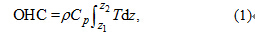
where ρ = 1029 kg m-3 is the density of sea water, Cp = 3901 J kg-1 K-1 is sea water specific heat capacity, z1, z2 are the depths of the vertical levels, and Tis sea water temperature.
Figure 1 shows the linear trends of surface wind stress (ZWS and MWS) anomalies and OSST anomalies for all six decades of the simulated period of 1949-2008. In general, all six decades show a warming trend and an anomalous westerly wind trend. The most significant warming decade is during 1969-78, and there is a trend of 0.5° C per decade over about half the area of the Southern Ocean domain (Fig. 1c). There are continuous westerly wind anomalies for the three decades from 1969 to 1998 (Figs. 1c-e). In the recent hiatus decade, OSST shows a slight warming trend, and there is little increase in the westerly anomalies (Fig. 1f). Note that the northward wind significantly increases in the southwest of South America in the recent hiatus decade (Fig. 1f). Both the wind stress trend and OSST trend are significant in most decades (Figs. 1a-e), which indicates that the anomalies of wind stress and thermohaline forcing both play a role in forcing the model in Exp_all. The areas of anomalous wind stress vectors and anomalous OSST do not overlap. Thus, there may be few nonlinear interactions in Exp_all when they both contribute to heat exchange between the water mass and the overlaying atmosphere. Furthermore, it is reasonable to consider wind stress and thermohaline forcing individually (Table 1, Exp_ws, and Exp_th). Because there is no sea ice process in our model, and the surface salinity gradient in the Southern Ocean is small, the buoyancy flux anomaly is caused mainly by the surface temperature anomaly. In addition, DHF is the combination of solar radiation, longwave radiation, latent heat flux, and sensible heat flux. The uncertainty of DHF is larger than that of OSST (Large and Yeager, 2008). For this reason, we chose OSST, instead of DHF, to examine the trend of surface thermohaline forcing.
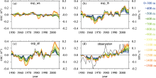
Following Chen and Tung (2014), we examined the OHC per 100 m in the upper 1500 m of the Southern Ocean. Figure 2 shows the simulated OHC from all three experiments (Figs. 2a-c). The observations from Ishii and Kimoto (2009) are also shown for comparison (Fig. 2d). It is apparent that the observed SST shows a slight trend in the recent hiatus decade, consistent with Fig. 1f. The anomalies for both OHC and SST in all panels refer to the whole period of 1949-2008. Since Exp_all included all the surface forcings, it can represent the model’ s ability in simulating the heat sink (Fig. 2c). The amplitude of the simulated OHC anomaly is larger than that observed (Fig. 2c). Nevertheless, the model simulated a heat sink well in the Southern Ocean in the recent hiatus decade. In the period 1960-70, the model simulates more heat variation than observed in the deeper layers (Fig. 2c). Keep in mind that the observational data before 1970 are not as reliable as in the later period (Ishii and Kimoto, 2009). In addition, observations in deeper layers are much more sparse for the period before the 1970s than after. The SST anomaly (SSTA) reaches its minimum at around 1960, but the observed heat change is not significant in deeper layers at that time (Fig. 2d). This may be due to the lack of data in the deeper layers. In contrast, the model heat sink is apparent in the period 1960-70, as inferred from the wide range of deeper OHC curves (Fig. 2c). The magnitude of the simulated SSTA is smaller than that observed (Figs. 2b and 2c). Note that the simulated SST is actually the upper-layer-averaged temperature. It is reasonable that the simulated SSTA is less variable than that observed.
 | Figure 1 Linear trends of observed sea surface temperature (OSST) (shading) and wind stress forcing (vectors) in the Southern Ocean for the six decades over the period 1949-2008. The shaded regions and vectors are statistically significant at 0.05 level according to the Student’ s t-test. The northern boundary in all panels is at 30° S. Latitude and longitude grid lines are at 30° intervals. The blue circle in (a) indicates the boundary of the Southern Ocean; the border latitude is 35° S. |
| Table 1 Details of the three experiments carried out in this study. The seven forcing variables (ZWS, MWS, SLP, OSST, OSSS, EMP, and DHF) are described in detail in section 2. |
 | Figure 2 Integrated ocean heat content (OHC) from the surface to different indicated depths in the Southern Ocean for (a) Exp_ws, (b) Exp_th, (c) Exp_all, and (d) observation. Shown is the yearly mean deviation for the whole period for each layer. Color lines show the OHC (left y-coordinate). The black line shows the SSTAs (right y-coordinate). |
Figure 2 also shows the relative contributions of wind stress and thermohaline forcing. The heat exchange between the ocean and the atmosphere is caused mainly by thermohaline forcing in the upper 600 m (Fig. 2b), while the contribution from wind stress forcing is weak in that layer (Fig. 2a), especially in the recent hiatus decade. Below 600 m, wind stress forcing plays a more important role, especially in the significant heat sink after 1999 (Fig. 2a). It should be noted that the 600 m is model specific, and also depends on vertical mixing schemes. The different contributions of these two types of forcing may be due to different physical processes for the heat budget. In the thermohaline forcing, heat exchange between the ocean and atmosphere is fast and effective, so vertical mixing processes dominate the heat budget. Although thermohaline forcing is essential in maintaining the Atlantic Meridional Overturning Circulation (AMOC), 60 years is not long enough for a significant change in the AMOC, so the heat exchange between the Atlantic and the Southern Ocean in deeper layers is not apparent compared to the upper layers. In the case of wind stress forcing only (Fig. 2a), the heat budget is maintained mainly by the adiabatic processes of horizontal advection. The anomalous westerly wind stress (Fig. 1) can give rise to an equatorward Ekman transport, which transports warm surface waters out of the Southern Ocean. Thus, wind stress anomalies do not give rise to an apparent heat sink in the upper layers. The heat gain of Fig. 2a in deeper layers after 1999 may be associated with an influx of water from the Pacific Ocean, which is caused by the Sverdrup dynamics as a result of the non-local effects of the wind stress. The apparent heat sink in Fig. 2a in the recent hiatus decade matches the observation well, which indicates that wind stress forcing may strengthen the heat sink in the deeper ocean during this period. Note that Fig. 2c can be seen as a linear combination of Figs. 2a and 2b. This is consistent with the analysis of Fig. 1, and further confirms that the separation of wind stress and thermohaline forcing is a reasonable approach, and their nonlinear interaction is weak. Another important difference between Fig. 2a and 2b occurs in the SSTA fields. The amplitude of SSTA in Exp_ws is much smaller than that in Exp_th. This is because the model SST was damped back to OSST (with a time scale of 120 days), OSST was the seasonal cycle climatology in Exp_ws (Fig. 2a), while in Exp_th it was composed of monthly mean values.
We investigated the heat sink in the Southern Ocean in the recent hiatus decade through three OGCM experiments, with different surface forcing strategies. The combined and individual contributions of wind stress and thermohaline forcing were examined. The results showed that thermohaline forcing is dominant in the heat exchange between the Southern Ocean and its overlaying atmosphere in the upper layers. In intermediate layers, wind stress forcing plays a more important role. In particular, wind stress forcing has strengthened the heat sink introduced by thermohaline forcing in the deeper ocean during the recent hiatus decade. The three experiments also showed that, in the simulated period of 1949-2008, the contributions of wind stress and thermohaline forcing can be seen as a linear combination of the heat exchange between the Southern Ocean and its overlaying atmosphere. The mechanism for the different contributions of the two types of forcing may be due to different physical processes for the heat budget. In the thermohaline forcing, the heat budget is maintained mainly by vertical mixing in the upper layers, while in the wind stress forcing it is maintained mainly by Ekman transport and Sverdrup dynamics. Since the results presented in this paper all derive from OGCM experiments, further investigations, either theoretical or observation-based, are needed to verify these numerical results.
Another limitation of this study is the lack of sea ice in the model, since the sea ice process is important for deep convection in the Southern Ocean. It can introduce significant change in sea surface salinity. Further analysis of the buoyancy flux anomalies could improve understanding of the heat exchange between the Southern Ocean and the overlaying atmosphere, and the associated climatic effects of such heat exchange.
| 1 |
|
| 2 |
|
| 3 |
|
| 4 |
|
| 5 |
|
| 6 |
|
| 7 |
|
| 8 |
|
| 9 |
|
| 10 |
|
| 11 |
|
| 12 |
|
| 13 |
|
| 14 |
|
| 15 |
|
| 16 |
|
| 17 |
|
| 18 |
|
| 19 |
|
| 20 |
|
| 21 |
|