
Modeling of Arctic Sea Ice Variability During 1948-2009: Validation of Two Versions of the Los Alamos Sea Ice Model (CICE)
[WU Shu-Qiang1, 2 , ZENG Qing-Cun3 , BI Xun-Qiang1, *  ]
]
]
|
|


The Los Alamos sea ice model (CICE) is used to simulate the Arctic sea ice variability from 1948 to 2009. Two versions of CICE are validated through comparison with Hadley Centre Global Sea Ice and Sea Surface Temperature (HadISST) observations. Version 5.0 of CICE with elastic-viscous-plastic (EVP) dynamics simulates a September Arctic sea ice concentration (SASIC) trend of -0.619 × 10¹² m2 per decade from 1969 to 2009, which is very close to the observed trend (-0.585 × 10¹² m2 per decade). Version 4.0 of CICE with EVP dynamics underestimates the SASIC trend (-0.470 × 10¹² m2 per decade). Version 5.0 has a higher correlation (0.742) with observation than version 4.0 (0.653). Both versions of CICE simulate the seasonal cycle of the Arctic sea ice, but version 5.0 outperforms version 4.0 in both phase and amplitude. The timing of the minimum and maximum sea ice coverage occurs a little earlier (phase advancing) in both versions. Simulations also show that the September Arctic sea ice volume (SASIV) has a faster decreasing trend than SASIC.
The Arctic sea ice has been undergoing an accelerated retreat in recent decades (Stroeve et al., 2012). Specifically, the rapid declining of the Arctic summer sea ice extent is mainly caused by surface warming, and is closely connected with the impacts of anthropogenic forcing. Sea ice plays an important role as a barrier separating the ocean from the atmosphere, acting as a communication bridge between the two. As sea ice melts, the ocean absorbs more, and reflects less, solar radiation, because of the great difference in albedo between with and without sea ice. At the same time, direct exchange of heat between the ocean and atmosphere takes place.
To date, there has been much research conducted on the role of sea ice in climate change due to global warming, and its amplification effect via the ice-albedo feedback mechanism (Arctic amplification). Screen and Simmonds (2010) found that diminishing sea ice has played a leading role in recent Arctic temperature amplification. Liu et al. (2012) investigated the correlation of Northern Hemisphere winter snowfall with the September Arctic sea ice retreat. Li and Wang (2014) demonstrated a significant change in the early 1990s in the relationships of the autumn Eurasian snow depth and the autumn Arctic sea ice cover with the East Asian winter monsoon. Vihma (2014) reviewed previous studies on the local and remote effects of the sea ice decline on weather and climate, and analyzed the dynamic processes by which sea ice decline can affect surface temperature, atmospheric circulation, and moisture.
The sea ice model is an important tool used for the polar regions. There is a long history of sea ice model development, from the early, simpler models, to more recent complex models. In terms of the thermodynamics, sea ice was originally modeled by simply including the sea ice albedo effect. Subsequently, many complex details have been considered, such as the ice thickness distribution and melt pond. For the dynamical aspects, sea ice was initially treated as a viscous-plastic (VP) material (Hibler, 1979, 1980). Since then, however, there have been many further studies on sea ice dynamics, for instance on cavitating fluid dynamics, free drift dynamics, and elastic-viscous- plastic (EVP) dynamics. Among the available sea ice models, the Los Alamos sea ice model (CICE) has the most complex physics parameterizations, and is the most widely used sea ice component model in coupled climate models. In this study, we aim to validate the improvements from version 4.0 to version 5.0 of CICE.
The paper is arranged as follows. In section 2, the model, data, and methods are described. In section 3, we perform a simple comparison among observed sea ice extents. In section 4, we analyze both the seasonal evolution and decadal variation of the sea ice simulation results. Section 5 is a summary and discussion.
The model employed in this research, CICE (Hunke et al., 2015), was designed to be a component of the National Center for Atmospheric Research (NCAR) Community Earth System Model (CESM). The present version of CICE used in NCAR CESM is version 4.0. Recently, the Los Alamos National Laboratory released CICE version 5.0, which has not yet been coupled into CESM. We use both versions in this study.
Compared with previous versions, CICE version 5.0 has been updated in a number of aspects; for example, two new melt pond parameterizations, sea ice biogeochemistry, and, of particular importance, a new dynamic elastic-anisotropic-plastic (EAP) rheology (Hunke et al., 2015). Different from the isotropic EVP rheology, the internal stress tensor described in EAP is related to the geometrical properties and orientation of underlying virtual diamond shaped floes (Wilchinsky and Feltham, 2006).
There are two dynamic options in CICE version 5.0: EVP rheology and EAP rheology. CICE version 4.0 only has EVP dynamics. In this study, to consider the different combinations in the two versions of CICE, we run five experiments, all of which are integrated from 1948 to 2009. The experiment details are listed in Table 1. All experiments use the thermodynamics model of Bitz and Lipscomb (1999) (hereinafter BL).
We take all the experiments with the standalone sea ice model, driven by the observed forcing data. The atmospheric forcing datasets are Common Ocean-ice Reference Experiments version 2 (CORE-v2), with interannual variation. The ocean forcing fields are set by CICE. All forcing datasets are interpolated into CICE tripolar grids.
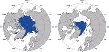
Figure 1 shows the Arctic region used in this study, with the distribution of sea ice coverage shaded in blue. There is significant change in the September Arctic sea ice coverage from 1970 to 2012. It is hard to simulate the precise sea ice distribution, because it depends on perfect initial conditions of both ocean and sea ice, and there is a predictability issue. So, our analyses just focus on the overall sea ice coverage.
To validate the CICE models, we use several available observations: (1) Hadley Centre Global Sea Ice and Sea Surface Temperature (HadISST), from 1880 to 2014; (2) National Oceanic and Atmospheric Administration (NOAA) Optimum Interpolation Sea Surface Temperature V2 (OISST2), from 1981 to 2014; and (3) the European Centre for Medium-Range Weather Forecasts (ECMWF) reanalysis products of the global atmosphere and surface conditions for 45-years (hereinafter ERA-40, from 1958 to 2001) and ERA-Interim (from 1979 to 2014). ERA-Interim data are generally regarded as the most reliable, but their availability covers a shorter period.
The Arctic sea ice concentration (hereinafter ASIC) plays an important role in regulating climate (Liu et al., 2012). Our focus is on the long-term trend of September ASIC (hereinafter SASIC). The Arctic sea ice volume (hereinafter SASIV) is another important factor (Schweiger et al., 2011), whose changes we also discuss.
| Table 1 Experiment design schemes. |
 | Figure 1 The Arctic sea ice coverage in September 1970 (left) and 2012 (right). The area, with sea ice fraction larger than 0.15, is shaded in blue. |
It is widely accepted that the recent rapid warming began around 1970, so we choose 1969-2009 as the period to calculate the trend and correlation. The percentage of the trend is calculated as the trend divided by the average of the first three years.
In this paper, the Arctic sea ice area (or extent, concentration) refers to the sea ice fraction multiplied by the actual grid area; the computing method is the same as in Liu et al. (2012). We only consider sea ice fractions larger than 0.15. The grid area (Sa) is calculated from latitude (ϕ ), longitude (φ ), and grid size ( 
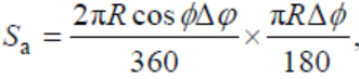
where R is the earth radius, and the sea ice volume is calculated from multiple sea ice areas by thickness.
There are several datasets of Arctic sea ice extent. Here, we study the consistency and availability of these datasets. As the Arctic temperature amplification is caused mainly by the declining sea ice (Screen and Simmonds, 2010), we calculate the negative correlation between 10 m temperature over the Arctic (hereinafter T10) and ASIC.
Figure 2 presents the SASIC of all the observational datasets, and the September Arctic 10 m temperature is also drawn (red line). We find that all the datasets are highly consistent with one another in the shared time periods. However, OISST has a higher SASIC than the others after the year 2000, and ERA-40 shows a slightly smaller SASIC than HadISST before 1980.
The correlation of observed September Arctic sea ice extent with 10 m temperature in the Arctic is also shown, as Cor (short for correlation) and Tr (short for trend), in Fig. 2. Because each observational dataset has a different time period, we calculate the correlations at different time scales, as shown in brackets in Fig. 2. We find that HadISST has the highest correlation (negative) with T10 and ERA-40 has the lowest. We also find that HadISST is similar to ERA-Interim, in both trend and correlation, with T10.
Because HadISST has the longest period and the highest correlation with T10, we choose the HadISST sea ice extent as the observation, and use it to compare with the model results in the following analysis.
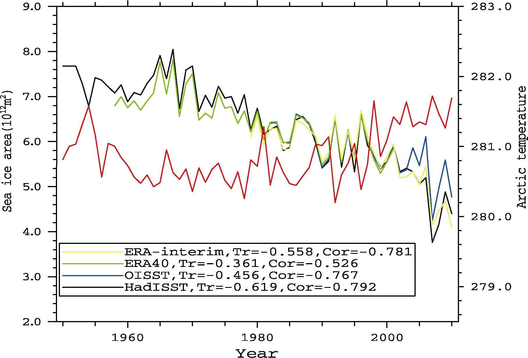 | Figure 2 Time series of the observed the September Arctic sea ice concentration (SASIC, units: 1012 m2) and T10 (units: K). Observed SASIC is shown in black (Hadley Centre Global Sea Ice and Sea Surface Temperature (HadISST)), blue (Optimum Interpolation Sea Surface Temperature (OISST)), green (ERA40), and yellow (ERA-interim). The red line is T10 from Common Ocean-ice Reference Experiments version 2 (CORE-v2). The correlation of observed SASIC with T10 and its trend are shown as Cor and Tr, respectively. |
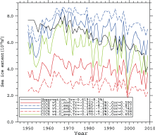
Figure 3 shows the simulated SASIC in all experiments listed in Table 1, and a comparison with HadISST observations. In the experiments without sea ice dynamics (experiments with the subscript “ _nod” ), the simulated SASIC in both versions is far away from the observation, and there is no declining trend. However, all experiments with dynamics have a turning point at around 1970, which is similar to the actual surface temperature changes. In the experiments with dynamics, SASIC grows before 1970, and then shows a declining trend, which is consistent with the HadISST observation. Comparing the two experiments with EVP dynamics, we note that the SASIC simulated by CICE version 5.0 (solid blue line) is closer to the observation (black line) than that of version 4.0 (green line).
The simulated SASIC’ s trends and correlations with the observation are also shown in Figure 3. The trend and correlation are calculated from 1969 to 2009, for the reason that SASIC has a mostly rising trend from 1948 to 1969. CICE version 5.0 with EVP dynamics simulates a SASIC trend of -0.585 × 10¹² m2 per decade from 1969 to 2009, which is very close to the observed trend (-0.619 × 10¹² m2 per decade). CICE version 4.0 with EVP dynamics underestimates the SASIC trend (-0.470 × 10¹² m2 perdecade). Furthermore, version 5.0 has a higher correlation (0.742) with the observation than version 4.0 (0.653). These improvements are mainly due to the implementation of new physics parameterizations, e.g., the melt pond parameterizations. However, the new EAP dynamics of CICE version 5.0 underestimates the declining trend, though the correlation is the highest among all experiments.
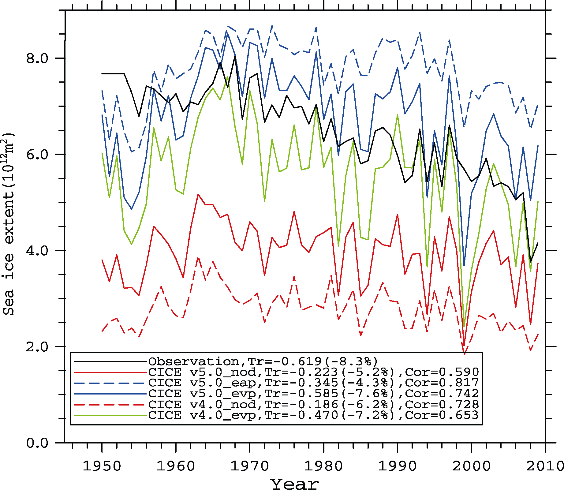 | Figure 3 Comparison of simulated September Arctic sea ice area (units: 1012 m2) from 1948 to 2009 with HadISST observations (black line). Simulated SASICs are shown as the blue solid line (CICE_v5.0_ evp), blue dashed line (CICE_v5.0_eap), red solid line (CICE_v5.0_nod), green solid line (CICE_v4.0_evp), and red dashed line (CICE_v4.0_ nod). The trend of SASIC from 1969 to 2009 (103 km3 per decade) and the correlation with HadISST are also shown, as Tr and Cor, respectively. |
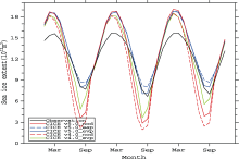
The annual cycle of ASIC is another important factor to assess the sea ice model’ s performance, especially the timing of the minimum and maximum sea ice coverage. The annual maxima of ASIC occur at the end of the frozen season (in later winter or early spring), and the minima occur at the end of the melt season (later summer or autumn).
Figure 4 shows the simulated three-year cycle of monthly ASIC, and a comparison with observations. The simulated seasonal cycle of ASIC is consistent with observations. In CICE version 4.0, the simulated timing of the minimum ASIC is in August instead of the observational September (phase advances), and the simulated amplitude is too large. CICE version 5.0 simulates larger than observed ASIC in all months. However, CICE version 5.0 (especially with EAP dynamics) shows an improvement in both phase and amplitude, compared with the HadISST observations.
For the experiments without dynamics (experiments with the subscript “ _nod” ), the simulated SASIC is too small during summer (melts and freezes too quickly), as in Fig. 3.
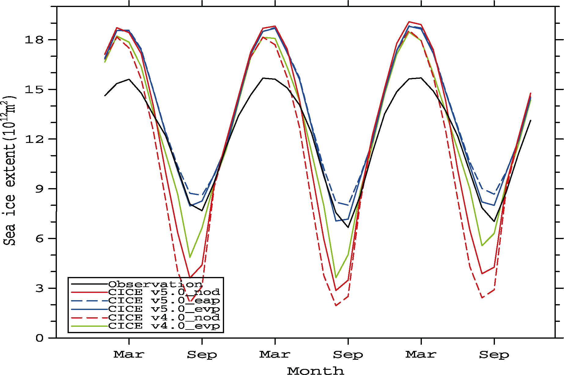 | Figure 4 Comparison of simulated three-year seasonal cycle of the Arctic sea ice area (units: 1012 m2) with HadISST observations (black line). Simulated SASICs are shown as the blue solid line (CICE_v5.0_ evp), blue dashed line (CICE_v5.0_eap), red solid line (CICE_v5.0_nod), green solid line (CICE_v4.0_evp), and red dashed line (CICE_v4.0_nod). |
Sea ice volume is decided by both area and thickness, and is a more sensitive factor than sea ice area with respect to global climate change. A specific change in sea ice volume would directly cause a corresponding change in heat latent. Moreover, global climate model simulations show that the trend in the Arctic sea ice volume exceeds the trend in sea ice extent; in other words, ice volume is a more sensitive climate indicator than ice extent. Unfortunately, there are fewer observational records of sea ice volume than of sea ice extent. However, by using a sea ice model, we can obtain long-term sea ice volume data for analysis.
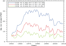
The simulated time series of SASIV in three experiments are presented in Fig. 5. As can be seen, we also find a turning point of SASIV at around 1970. Furthermore, the SASIV simulation results are more scattered than those of SASIC.
The SASIV trends in three experiments are also shown, as Tr, in Fig. 5. According to Schweiger et al. (2011), the Pan-Arctic Ice-Ocean Modeling and Assimilation System (PIOMAS) models an Arctic sea ice volume trend of (-2.8 ± 1) × 103 km3 per decade from 1980 to 2010. CICE version 5.0 (both EVP and EAP dynamics) is more consistent with PIOMAS than the other experiments, while CICE version 4.0 underestimates the trend. Furthermore, taking the experiments with EVP dynamics as a reference, the simulated trend of sea ice volume (more than -12% per decade) from 1969 to 2009 is more distinct than that of sea ice concentration (less than -9% per decade).
However, without dynamics, both versions of CICE simulate an increasing trend of SASIV, which is not logical. So, we don’ t show the results here.
 | Figure 5 Time series of simulated Arctic sea ice volume (units: 103 km3) in September from 1948 to 2009 in experiments CICE_v5.0_evp (blue line), CICE_v5.0_eap (green line), and CICE_v4.0_evp (red line). The trend of SASIV from 1969 to 2009 (103 km3 per decade) is also shown, as Tr. |
In this study, five experiments are conducted to compare two versions of CICE, and the main results demonstrate that the overall performance of CICE version 5.0 is better than CICE version 4.0.
Our focus is on the fields that are closely related to climate change issues, e.g., sea ice retreat, especially the long-term trend of September Arctic sea ice extent. CICE version 5.0 with EVP dynamics simulates a SASIC trend of -0.619 × 10¹² m2 per decade from 1969 to 2009, which is very close to the observed trend (-0.585 × 10¹² m2 per decade). CICE version 4.0 (EVP) underestimates the SASIC trend (-0.470 × 10¹² m2 per decade). Version 5.0 has a higher correlation (0.742) with observation than version 4.0 (0.653).
The long-term mean of the seasonal cycle of the Arctic sea ice extent is also considered. The results reveal that both versions of CICE simulate the annual cycle of Arctic sea ice, albeit the timing of the minimum and maximum sea ice coverage occurs a little earlier than observed (phase advancing). Furthermore, CICE version 5.0 outperforms CICE version 4.0 in both phase and amplitude.
Simulations of the SASIV reveal a more rapid decreasing of SASIV than SASIC, which agrees with the study of Schweiger et al. (2011). Without dynamics, simulated SASIV is not logical in both versions of the model.
To improve the simulation of the Arctic sea ice distribution, we plan to add an actual oceanic forcing and carry out further experiments. Upon completion of the validation of CICE version 5.0, we plan to implement it into a coupled climate model.
| [1] |
|
| [2] |
|
| [3] |
|
| [4] |
|
| [5] |
|
| [6] |
|
| [7] |
|
| [8] |
|
| [9] |
|
| [10] |
|
| [11] |
|