Arctic Oscillation Responses to Black Carbon Aerosols Emitted from Major Regions
[WAN Jiang-Hua1, 2 , LI Shuanglin1, *  ]
]
]
|
|


The responses of the Arctic Oscillation (AO) to global black carbon (BC) and BC emitted from major regions were compared using the atmospheric general circulation model Geophysical Fluid Dynamics Laboratory (GFDL) atmospheric general circulation model (AGCM) Atmospheric Model version 2.1 (AM2.1). The results indicated that global BC could induce positive-phase AO responses, characterized by negative responses over the polar cap on 500 hPa height fields, and zonal mean sea level pressure (SLP) decreasing while zonal wind increasing at 60°, with the opposite responses over midlatitudes. The AO indices distribution also shifted towards positive values. East Asian BC had similar impacts to that of global BC, while the responses to European BC were of opposite sign. South Asian BC and North American BC did not affect the AO significantly. Based on a simple linear assumption, we roughly estimated that the global BC emission increase could explain approximately 5% of the observed positive AO trend of +0.32 per decade during 1960 to 2000.
The extratropical atmospheric circulation of the Northern Hemisphere in winter is dominated by the Arctic Oscillation (AO), also referred to as the Northern Annular Mode (NAM), which is characterized by deep, zonally symmetric, or “ annular” structures, with synchronous fluctuations in pressure of one sign over the polar cap and of opposite sign at lower latitudes (Thompson and Wallace, 1998, 2000; Baldwin and Dunkerton, 2001). Previous studies have indicated that the North Atlantic Oscillation (NAO) is a regional manifestation of the AO variability (Thompson and Wallace, 1998; Thompson et al., 2000; Marshall et al., 2001).
Various indices related to the AO have exhibited a pronounced drift toward high index polarity during the last few decades of the 20th century, which is reflected in patterns of sea level pressure, geopotential height, and surface air temperature trends (Hurrell, 1996; Thompson and Wallace, 1998). Thompson et al. (2000) revealed that the AO/NAO had an increasing trend during the last few decades of the 20th century. Moreover, Feldstein (2002) suggested that the trend was significantly beyond that expected from internal variability of the atmosphere, and thus was due either to a coupling process or external forcing. Hoerling et al. (2004) attributed this significant positive trend to tropical ocean warming, principally Indian Ocean warming. Li et al. (2006) used a coupled model to demonstrate that local North Atlantic air-sea feedback could amplify the NAO response to the Indian Ocean warmth. Some other natural variability factors may also contribute to AO/NAO variations, such as ENSO, mega-ENSO (Wu and Zhang, 2014; Wu and Lin, 2012), and Arctic sea ice (Wu et al, 2011).
Allen and Sherwood (2011) suggested the AO could be influenced by global aerosol forcing. Robock (2000) and Shindell et al. (2004) showed that tropical volcanic aerosols can cause a positive AO anomaly. Chung and Ramanathan (2003) used CCM3 (Community Climate Model, version 3) experiments to find that the remote impacts of Southeast Asian haze may be associated with AO variability. Black carbon (BC) is thought to be the second-largest contributing agent to observed global warming from anthropogenic activities after carbon dioxide (Bond et al., 2013). Wang (2009) found that a substantial difference exists in the responses of the Intertropical Convergence Zone (ITCZ) to BC aerosols emitted from major regions. With increasing global emissions of BC (Bond et al., 2007; Cooke et al., 1999; Ito and Penner, 2005) during the last few decades of the 20th century, with East Asian BC emissions increasing particularly rapidly, whether or not the AO is affected by BC emissions over different regions, and to what extent BC emissions might be responsible for the AO trend, is intriguing. Such thoughts motivated the present study, which used an ensemble of atmospheric general circulation model (AGCM) simulations to investigate the responses of the AO to BC from various regions around the globe.
We repeated the ensemble sensitivity experiments in Wan et al. (2013) on another platform— namely, the Geophysical Fluid Dynamics Laboratory Atmospheric Model, version 2.1 (GFDL AM2.1) (Anderson et al., 2004)— and added several sets of companion sensitivity experiments. The model has a horizontal resolution of 2.5° longitude × 2° latitude, with 24 vertical levels in a hybrid coordinate grid. The aerosols were obtained from a chemical transport model, the Model for Ozone And Related Chemical Tracers (MOZART) (Horowitz et al., 2003).
Six sets of ensemble experiments, each consisting of five members, were performed. The control group (CTL) had historical evolution of aerosol burdens. Each of the five runs started in the first five days in January 1970, and were integrated to December 2000. As the model spin-up year, outputs of 1970 were not used. The sensitivity simulations involved the BC being maintained at the level in 1860 over the globe, Europe (35-65° N, 0° -60° E), East Asia (20-50° N, 100-130° E), South Asia (10-30° N, 70-100° E), and North America (25-55° N, 255-295° E), separately. The sectors represented the major BC emission regions around the globe (Wang, 2009). The sensitivity experiments are referred to as noGBC, noEUBC, noEABC, noSABC, and noNABC, respectively. All other model settings were identical to the CTL runs.
ERA-40 reanalysis data were also adopted, to verify the model’ s performance in terms of intrinsic variability. The responses to BC were the differences between the 30-year CTL average and the corresponding sensitivity ensemble.
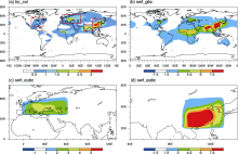
The difference of BC column burden between CTL and noGBC ensemble in boreal winter is illustrated in Fig. 1a. The large burden centers are highlighted with rectangles, which are also the fixed BC regions for the other four sensitivity experiments. The total difference of the BC amount was 215 Gg. The direct influence of BC is heating the air by strongly absorbing shortwave radiation (Jacobson, 2010). Figure 1 also presents the net shortwave radiative flux absorbed by BC in the atmosphere, calculated by subtracting the net shortwave radiative flux at the surface from that at the top of the atmosphere (TOA), in response to GBC, EUBC, and EABC. The distribution of the net BC absorbed shortwave radiative flux was similar to that of BC burden. The global BC absorbed shortwave radiative flux was +1.29 W m-2, and the maximum value was +10 W m-2 over East Asia, which is smaller in magnitude than that reported by Bond et al. (2013). As they pointed out, this could be attributed to the underestimation of the amount of BC in the atmosphere, as well as the imperfection of the treatment of the absorption caused by mixing of BC with other constituents.
 | Figure 1 (a) Black carbon (BC) column burden differences between the model’ s control (CTL) and noGBC ensembles (units: mg m-2). The rectangles represent the fixed BC regions in four companion sensitivity experiments. Simulated responses for net shortwave radiative flux absorbed by BC in the atmosphere (units: W m-2) to (b) GBC, (c) EUBC, and (d) EABC. |
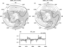
Figure 2a displays the structure of the AO mode in observation, which is defined as the leading empirical orthogonal function (EOF1) of monthly mean geopotential height anomalies for all months of the year at 500 hPa north of 20° N. It resembles the regression of 500 hPa heights against the time coefficient of the EOF1 of sea level pressure (SLP), which exhibits a more zonally symmetric structure on the hemispheric scale (Thompson and Wallace, 1998). The corresponding time series (PC1) is referred to as the AO index (Fig. 2b). In addition to somewhat episodic fluctuation, the AO index time series showed a drift toward the high value in the last 40 years of the 20th century. The linear trend for the period 1960 to 2000 was +0.32 per decade, which is comparable to the SLP-based AO index trend of +0.24 per decade during 1966 to 2004 (Cohen and Barlow, 2005). Other AO/NAO indices calculated with different methods also show a significant positive trend in the latter decades of the 20th century (Hurrell et al., 2004; Rodwell et al., 1999; Pinto and Raible, 2012).
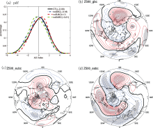
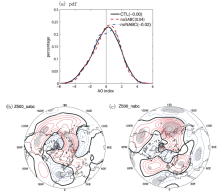
Figure 2c displays the leading EOF of 500 hPa heights in the control ensemble, which explains 17.8% of the total variance. The pattern resembles the observed AO (Fig. 1a), albeit showing a smaller amplitude, with -25 gpm over the negative center over Greenland compared to -35 gpm in observation. Nevertheless, the pattern correlation coefficient between them reached 0.9, verifying the model’ s ability to simulate the intrinsic variability as the AO. The AO indices of different experiments were obtained by projecting the corresponding 500 hPa geopotential height anomalies, relative to a 1971-2000 base period of the control ensemble, onto the leading EOF pattern in the control run. Figure 3a shows the estimated probability density function (PDF) of the AO indices in CTL, noGBC, noEUBC, and noEABC during the winter months. The PDF of the AO indices showed a normal distribution, with a mean value of 0 in the CTL ensemble. However, the distribution under both noGBC and noEABC conditions exhibited shifts toward the negative AO phase, with mean values of -0.18 (± 0.19) and -0.21 (± 0.17), respectively. The ensemble standard deviations in parentheses indicate substantial uncertainty of the responses. On the contrary, the distribution of the noEUBC ensemble shifted toward the positive phase, with a mean value of +0.17 (± 0.19). The differences of the AO mean values between the CTL ensemble and the three sensitivity experiments all passed the significance test at 0.1 level, giving confidence to GBC and EABC being able to induce positive AO responses, and EUBC a negative AO response.
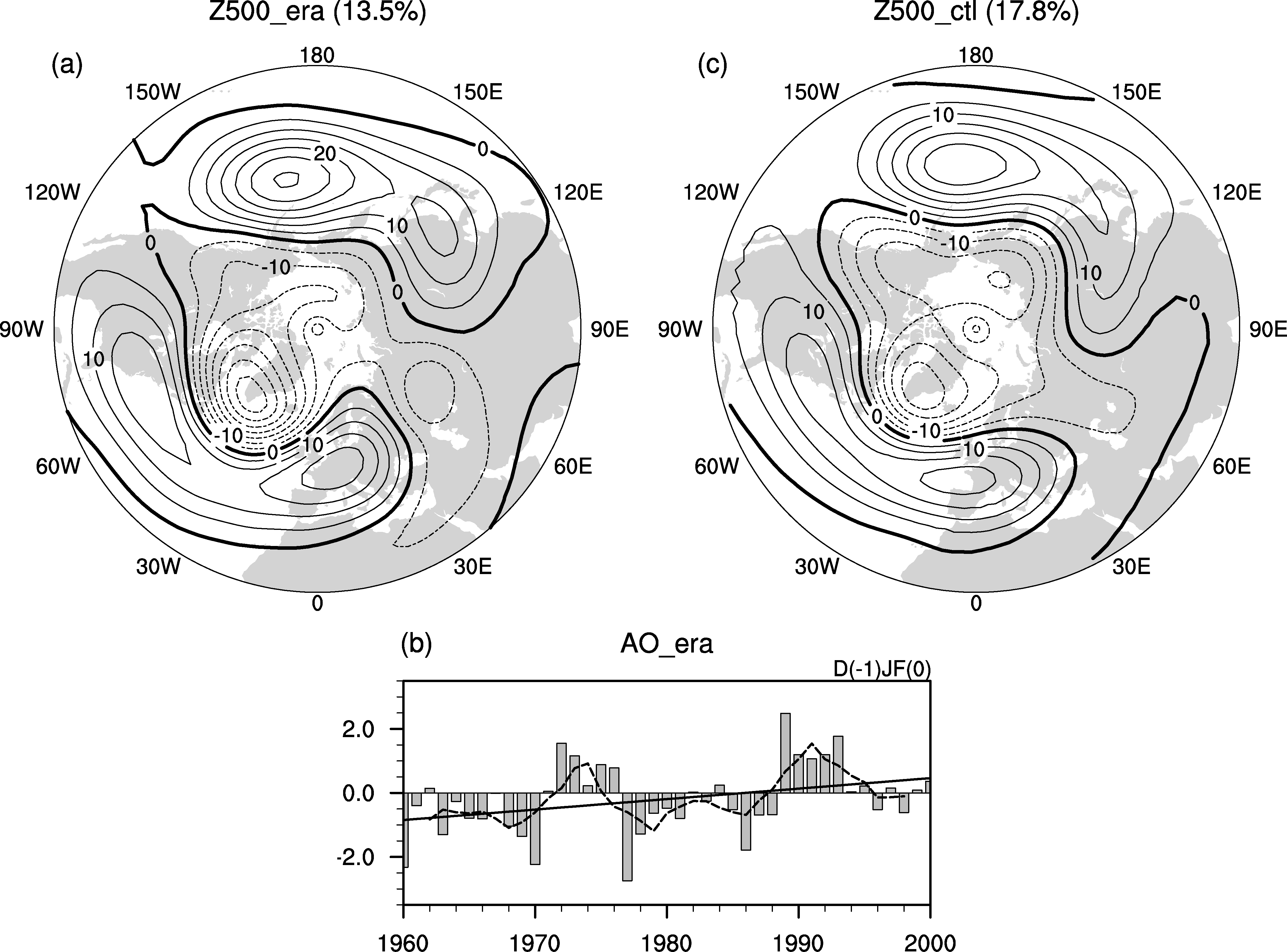 | Figure 2 (a) Leading empirical orthogonal function (EOF1) of the year-round monthly mean 500 hPa geopotential height anomalies over the Northern Hemisphere (20-90° N) and (b) the wintertime (DJF) seasonal mean of the corresponding time series in ERA-40 reanalysis data. (c) EOF1 of the 500 hPa height poleward of 20° N in the control ensemble. Numbers in parentheses in (a, c) represent the percentage of the total variance they explain. The contour increment is 5 gpm in (a, c). Dashed lines in (a, c) represent negative values. Bars in (b) represent the average of the DJF indices for each year; the dashed line represents the five-year smoothed indices; and the solid line represents the linear trend of the series. |
The results are manifested in the differences of 500 hPa geopotential heights between CTL and the sensitivity ensembles, as shown in Figs. 3b-d. GBC caused negative responses that were mainly confined to the Arctic, with a central value of -8 gpm, and circumglobal positive responses over the midlatitude region. The four positive centers of action were generally in the same location as the observed AO mode, but the response over the North Pacific was relatively stronger than in other regions. The correlation coefficient between the responses and the leading EOF pattern in CTL was +0.69, indicating the response forced by GBC was strongly projected onto the positive AO mode. This is consistent with a similar response to global anthropogenic aerosol forcing (Allen and Sherwood, 2011), which is composed of a high proportion of absorbing aerosols such as BC. The 500 hPa height response to EABC was remarkably similar to GBC in structure, with a pattern correlation coefficient up to 0.70, and even stronger in magnitude, with a -12 gpm negative center over Greenland. Thus, EABC also excited a positive AO pattern response, which is in agreement with a specified heating experiment result using Community Atmosphere Model (CAM) (Teng et al., 2012). The responses to EUBC, on the other hand, showed weaker magnitude and opposite sign to those of GBC and EABC. The correlation coefficients between the AO pattern in CTL and the EABC and EUBC responses were 0.67 and -0.61, respectively.
 | Figure 3 (a) Probability distribution function (PDF) of the Arctic Oscillation (AO) indices in the CTL, noGBC, noEUBC, and noEABC experiments, with mean values in parentheses. Simulated responses for geopotential height at 500 hPa (units: gpm) to (b) GBC, (c) EUBC, and (d) EABC. The contour increment is 2 gpm. Dashed lines in (b-d) represent negative values. Shadings represents the 90% confidence level using the t-test. |
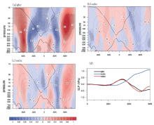
The zonal symmetry signature of the AO can be well characterized by out-of-phase variations in westerly momentum in the ~35° and ~60° latitude belt, as well as in the atmospheric mass between the polar cap regions poleward of 60° and the surrounding zonal rings centered near 45° (Thompson and Wallace, 2000; Baldwin et al., 1994; Baldwin and Dunkerton, 1999). Figure 4 shows zonally averaged zonal wind and SLP in response to GBC, EUBC, and EABC. GBC increased the zonal wind near 60° N throughout the troposphere and lower stratosphere, while decreasing that near 30° N. This, as in Allen and Sherwood (2011), is a reflection of an enhanced AO mode. Besides, the responses also exhibited an inter-hemispherical symmetric feature, implying GBC may exert a similar impact on the Antarctic Oscillation (AAO), but this was beyond the scope of the current study. A similar pattern with relatively smaller magnitude was forced by EABC, and an opposite pattern was forced by EUBC. Moreover, Fig. 4d shows that GBC and EABC induced similar SLP changes at high latitudes; that is, negative responses poleward of 60° N, both peaking at -0.5 hPa, while EUBC had a significant positive response at high latitudes. The GBC/EABC and EUBC impacts on zonal wind and SLP were reminiscent of positive and negative AO, respectively (Thompson and Wallace, 2000).
Unlike the distribution of the AO indices shifting far away from the neutral state under noGBC, noEABC, and noEUBC conditions, the corresponding mean values of AO indices were 0.04 (± 0.25) and -0.02 (± 0.23) for noSABC and noNABC, respectively, neither of which passed the significance test at 0.15 level (Fig. 5a). The 500 hPa geopotential height responses to SABC and NABC exhibited a more zonally asymmetric component (Fig. 5). It appears that BC over South Asia and North America do not exert significant impacts on the AO pattern. The maximum central value of BC column burden differences over North America was 1.3 mg m-2, while the maximum central value over East Asia was 3.5 mg m-2. It is possible that, in this study, the relatively weak forcing over North America could not induce significant AO responses.
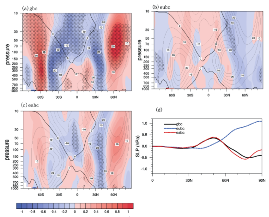 | Figure 4 Simulated responses for zonal-mean zonal wind (units: m s?1) to (a) GBC, (b) EUBC, and (c) EABC. (d) Simulated responses for zonally averaged sea level pressure (units: hPa) to the sensitivity runs. In (aCc), shadings represents the responses; contours represent the climatological zonal wind calculated from the CTL ensemble; and dashed lines represent negative values. Black dots represent the 90% confidence level. |
 | Figure 5 (a) PDF of the AO indices in the CTL, noSABC and noNABC experiments, with mean values in parentheses. Simulated responses for geopotential height at 500 hPa (units: gpm) to (b) SABC and (c) NABC. The contour increment is 2 gpm. Dashed lines in (bCc) represent negative values. Shadings represents the 90% confidence level using the t-test. |
We compared the impacts of GBC, EUBC, EABC, SABC, and NABC on the AO using GFDL AM2.1. The results indicated that GBC could force positive-phase AO responses characterized by negative responses over the polar cap, as well as positive responses over midlatitudes on 500 hPa geopotential height fields, in accordance with the zonal mean SLP (zonal wind) decreasing (increasing) at 60° and decreasing (increasing) at mid-low latitudes. Besides, the PDF of the AO indices shifted towards negative values, with a mean value of -0.18 (± 0.19) under the noGBC condition. The responses to EABC were similar to those of GBC, albeit with larger amplitude, while the responses to EUBC were of opposite sign. The impacts of SABC and NABC did not project on the AO pattern.
During the last few decades of the 20th century, the AO indices showed an upward trend of +0.32 per decade. Meanwhile, global BC emissions kept increasing (Cooke et al., 1999; Ito and Penner, 2005; Bond et al., 2007), of which the BC over East Asia increased particularly rapidly during the latter half of the 20th century due to the development of the economy (Bond et al., 2007). As stated earlier, the AO index distribution shifted from 0.0 to +0.18 in response to a total of 215 Gg BC burden forcing. According to the GFDL model estimation, the linear trend of the global total BC burden during 1960 to 2000 was +19.9 Gg per decade. Thus, the amount of the AO index trend in linear agreement with the BC increase during the last 40 years of the 20th century was +0.017 per decade, accounting for approximately 5% of the observed positive AO trend during 1960 to 2000. This is a rough estimate based on a simple linear assumption; further work is needed to obtain more precise and robust results. EABC played the most important role in the BC induced AO trend, which could account for approximately 9% of the observed AO trend. EUBC would offset the impacts, while SABC and NABC do not affect the AO significantly.
Other important caveats to this study include the fact that we only applied one AGCM in this work. It is vital to assess the conclusions with coupled models. Also, the BC dataset used in this study was from a chemical model. Although the aerosol climatologies have been found to be in general agreement with observations (Ginoux et al., 2006; Horowitz, 2006; Tie et al., 2005), more experiments with different BC datasets are needed to evaluate the sensitivity of the forcing data to the conclusions.
| [1] |
|
| [2] |
|
| [3] |
|
| [4] |
|
| [5] |
|
| [6] |
|
| [7] |
|
| [8] |
|
| [9] |
|
| [10] |
|
| [11] |
|
| [12] |
|
| [13] |
|
| [14] |
|
| [15] |
|
| [16] |
|
| [17] |
|
| [18] |
|
| [19] |
|
| [20] |
|
| [21] |
|
| [22] |
|
| [23] |
|
| [24] |
|
| [25] |
|
| [26] |
|
| [27] |
|
| [28] |
|
| [29] |
|
| [30] |
|
| [31] |
|
| [32] |
|
| [33] |
|
| [34] |
|
| [35] |
|