The Connection between the Sea Surface Height Anomaly Preceding the Indian Ocean Dipole and Summer Rainfall in China
[DUAN Xin-Yu1, 2 , LIU Na2, 3, 4, *  , LI Shuanglin
2, 3 ]
, LI Shuanglin|
|


The sea surface height anomaly (SSHA) signals leading the fall Indian Ocean Dipole (IOD) are investigated. The results suggest that, prior to the IOD by one year, a positive SSHA emerges over the western-central tropical Pacific (WCTP), which peaks during winter (January-February-March, JFM), persists into late spring and early summer (April-May-June, AMJ), and becomes weakened later on. An SSHA index, referred as to SSHA_WCTP, is defined as the averaged SSHA over the WCTP during JFM. The index is not only significantly positively correlated with the following-fall (September-October-November, SON) IOD index, but also is higher than the autocorrelation of the IOD index crossing the two different seasons. The connection of SSHA_ WCTP with following-summer rainfall in China is then explored. The results suggest that higher (lower) SSHA_ WCTP corresponds to increased (reduced) rainfall over southern coastal China, along with suppressed (increased) rainfall over the middle-lower reaches of the Yangtze River, North China, and the Xinjiang region of northwestern China. Mechanistically, following the preceding-winter higher (lower) SSHA_WCTP, the South Asia High and the Western Pacific Subtropical High are weakened (intensified), which results in the East Asian summer monsoon weakening (intensifying). Finally, the connection between SSHA_WCTP and El Niño-Southern Oscillation (ENSO) is analyzed. Despite a significant correlation, SSHA_WCTP is more closely connected with summer rainfall. This implies that the SSHA_WCTP index in the preceding winter is a more effective predictor of summer rainfall in comparison with ENSO.
As a phenomenon that arises from regional air-sea interaction and is characterized by a strong zonal sea surface temperature anomaly (SSTA) gradient, the Indian Ocean Dipole (IOD) mode has been widely studied since the late 20th century (Saji et al., 1999). The IOD may influence summer climate over East Asia (Saji and Yamagata, 2003a; Tang et al., 2008; Zhao et al., 2009). During the developing years of positive-phase IOD events, enhanced rainfall emerges over southern China while there is reduced rainfall over northern China (Xiao et al., 2002), and vice versa. Therefore, identifying earlier signals to predict the IOD’ s formation is of substantial importance for East Asian climate prediction (Saji and Yamagata, 2003b; Izumo et al., 2010).
IOD events can be seen in sea surface height (SSH) anomalies and, as such, the SSH anomaly is often used as a proxy for the IOD (Aparna et al., 2012; Yuan et al., 2013). Furthermore, oceanic dynamical processes including flow advection, vertical entrainment, and upwelling (Behera et al., 1999), which may play an important role in the IOD’ s formation (Saji and Yamagata, 2003a), can to some extent be reflected in SSH. This is verified by the high correlation between SSH and the IOD (Rao et al., 2002; Feng and Meyers, 2003). In addition, the Indonesian Throughflow (ITF), which is driven by the SSH gradient along the Indian Ocean and equatorial Pacific (Du and Fang, 2011), can be a precursor to the IOD (Yuan et al., 2011). These results suggest the possible existence of earlier IOD signals in the SSH.
If earlier IOD signals in the SSH exist, a related issue is whether SSH can act as a predictor of summer rainfall in view of the IOD’ s substantial impacts. This is the primary motivation behind the present study, which aims to address the following questions: Can any significant SSH signal be found in advance that is linked to subsequent IOD events? If yes, how are the signals related to summer rainfall in China? These issues are currently not very well understood (Li et al., 2011).
The variables analyzed here include precipitation, sea surface temperature, sea surface height, and atmospheric circulation variables. The summer precipitation is from the gauged monthly dataset from 1951 to 2014 at 160 stations obtained from the National Meteorological Information Center of the China Meteorological Administration. The monthly extended reconstruction of global sea surface temperature (ERSST) data comes from National Oceanic and Atmospheric Administration (Smith et al., 2007) and is available online at http://www.cdc.noaa.gov/cdc/data.noaa.ersst.html. The SSH is from the National Centers for Environmental Prediction (NCEP) Global Ocean Data Assimilation System (GODAS; Behringer and Xue, 2004) covering the period from 1980 to 2014, which has a resolution of 1° in the east-west direction and (1/3)° in the north-south direction. The atmospheric circulation dataset is from the European Centre for Medium-Range Weather Forecasts Interim Reanalysis (ERA-Interim) datasets (Dee et al., 2011), which have a horizontal resolution of 0.75° × 0.75° and cover the period from 1979 to present.
Following Saji et al. (1999), the IOD index is defined as the difference in averaged SSTA between the western (10° S-10° N, 50-70° E) and eastern (10° S-0° , 90-110° E) equatorial Indian Ocean. Since the IOD peaks in fall, the IOD index in this study is denoted as the mean of SON.
Given that the IOD is significantly correlated with ENSO, and the positive-phase IOD tends to co-occur with El Niñ o and vice versa (Annamalai et al., 2005; Kug et al., 2006; Izumo et al., 2010), the connection between SSH and ENSO is also analyzed. ENSO is represented by the well-known Niñ o 3.4 index, i.e., the averaged SST anomaly over (5° S-5° N, 170-120° W).
The analysis period is 34 years from January 1981 to November 2014. Monthly anomalies are computed from each monthly mean by subtracting the climatological seasonal cycle. For each monthly variable, linear detrending is applied beforehand. Then, interdecadal variability with periodicities longer than seven years is removed through fast Fourier transformation. Saji and Yamagata (2003a) demonstrated that this filter can slightly improve the correlations of the SST between the eastern pole and western pole consisting of the IOD. The Student’ s t-test is applied for checking the significance of the results. Following the methodology of Wang et al. (2009), the significance is derived with decreased effective degrees of freedom. Since the decadal variability with periodicities longer than seven years is removed, the freedom of variables on the decadal timescale is defined as N/7-1. Then, the freedom for the interannual variability is defined as the subtraction of the freedom on decadal timescales from the total sample: N-(N/7-1), where N denotes the total sample number.
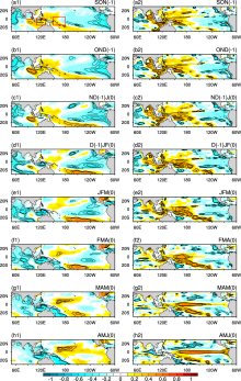
First, we try to identify the SSH signals in preceding periods that can be strongly associated with IOD events in fall. Thus, the relationships between the SSHA in preceding seasons and the IOD are investigated. Figure 1 shows a comparison of the correlations of the preceding SSHA and SSTA with the IOD. It is found that the SSHA and SSTA lead the IOD by 5 to 12 months from the preceding fall (SON(-1)) to the late-spring to early summer (AMJ(0)). Each month is presented as a three-month smoothed season. Based on this, the SSHA exhibits significantly higher leading correlations with the IOD than the SSTA. In comparison, the SSTA leading correlations are less significant. High correlations between the SSHA and IOD are primarily situated in several regions including the Bay of Bengal (BoB), the Maritime Continent (MC) and the western-central tropical Pacific (WCTP: the west to the dateline). These are further seen from the correlations between the averaged SSHA over these regions and the IOD (Table 1). The averaged SSH in these regions is expressed as “ SSHA_BoB” , “ SSHA_MC” , and “ SSHA_ WCTP” , respectively.
 | Figure 1 Distributions of correlation coefficients of the preceding (a1-h1) sea surface height anomaly (SSHA) and (a2-h2) the sea surface temperature anomaly (SSTA) with the September-October-November (SON) Indian Ocean Dipole (IOD) index during the period 1981-2014. The contours represent correlations significant above the 95% confidence level. |
| Table 1 Correlation coefficients of the area-averaged preceding the sea surface height anomaly (SSHA) over the selected regions with the September-October-November (SON) Indian Ocean Dipole (IOD) for the period 1981-2014. The fifth column shows the autocorrelations of the IOD with the leading months from 6 to 11. The bold values indicate significance at the 95% confidence level for the SSHA-lead and less significance for the SSTA-lead correlations. |
The positive correlations of the SSHA over the BoB are significant from the preceding fall to winter, with the maximum in SON(-1). In comparison, the SSTA correlations are insignificant during the same season. Over the MC region, the SSHA correlations persist from the preceding fall (SON(-1)) to winter (JFM(0)), with the maximum in the preceding fall and a decrease along with the seasonal march. In contrast, the strongest correlations of the SSTA in the region occur after the preceding winter.
The correlation between the SSHA over the WCTP region and the IOD are significant from the preceding fall (SON(-1)) to the late-spring-early-summer (AMJ(0)). The correlation achieves highest values in the WCTP during JFM(0) and shifts zonally to the eastern tropical Pacific. However, the SSTA correlations in these months are insignificant. This implies that the SSHA in this region may provide an early warning signal for the development of the following-fall IOD relative to the SSTA.
Whether the correlation between the preceding-fall SSHA_WCTP and the following fall IOD is higher than the across-seasonal autocorrelations of the IOD is key for the application of this finding. Thus, the lead-lag autocorrelations of IOD indices are also given in Table 1 (fifth column). Although significant negative autocorrelation (less than -0.4) persists from the preceding fall to winter, the autocorrelations become less significant after the preceding winter. From the preceding JFM(0) to AMJ(0), the autocorrelation of the IOD is very weak. This suggests that the preceding spring SSHA over the WCTP is a better signal than the IOD index itself in predicting the following-fall IOD events.
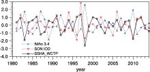
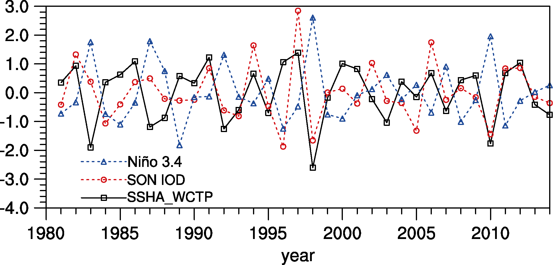 | Figure 2 Comparison of the evolution of the preceding January-February-March (JFM) SSHA_WCTP index (black line) and Niñ o 3.4 index (blue line) with the SON IOD index (red line) for the period 1981-2014. |
The fact that the SSHA over the WCTP from JFM(0) to AMJ(0) is more closely connected with the following-fall IOD is also seen in Fig. 2, which shows the historical evolution of JFM SSHA_WCTP and the following-fall IOD index from 1981 to 2014. The correlation between the two indices reaches a positive value of 0.46. Besides, the correlations of SSHA_WCTP in several other months (February-March-April (FMA) to AMJ) are also significant.
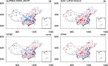
Figure 3a shows the correlation between following- summer rainfall in China and preceding-winter SSHA_ WCTP index. The gauged rainfall data from mainland China are used. Significant negative correlations appear over the middle-lower reaches of the Yangtze River, North China, and the Xinjiang region of Northwest China,
while positive correlations are situated over southern coastal China. Statistical calculation suggests a total number of 39 stations passing the significance test at the 90% confidence level.
To check the robustness of the above SSH-rainfall connection, composite analysis is conducted for higher/lower SSH_WCTP index years. The years are selected when the SSHA_WCTP index is greater (less) than one positive (negative) standard deviation. Thus, six higher index years (1986, 1991, 1996, 1997, 2000, and 2012)and six lower index years (1983, 1987, 1992, 1998, 2003, and 2010)are chosen (Fig. 2).
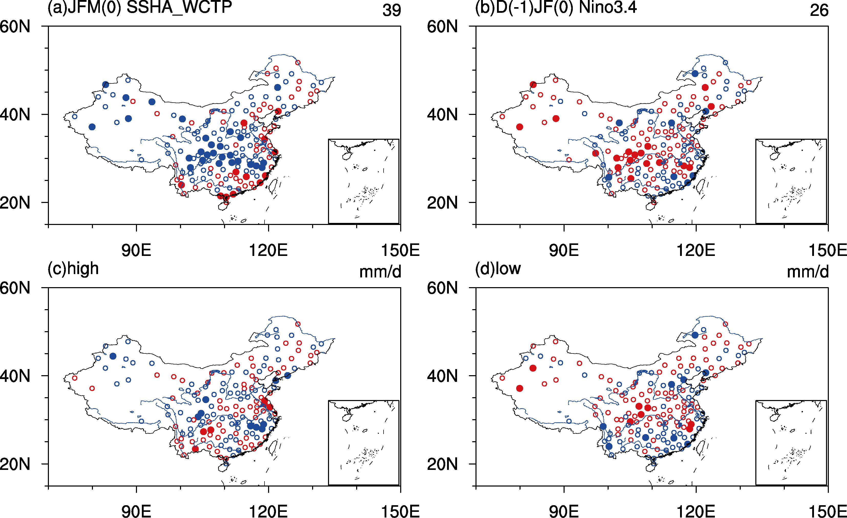 | Figure 3 Upper panels: correlation of summer rainfall at 160 stations within mainland China with (a) JFM SSHA_WCTP index and (b) simultaneous Niñ o 3.4 index. Only the sign and significance of the correlation coefficients are displayed. Filled (open) circles denote significance (insignificance) at the 90% confidence level, and red (blue) coloring represents a positive (negative) relationship. Lower panels: composite of observed summer rainfall anomalies (units: mm d-1) derived from the years with (c) high preceding-winter SSHA_WCTP index and (d) low preceding-winter SSHA_WCTP index. |
From Fig. 3c, the composite following-summer rainfall anomalies during higher SSHA_WCTP years display a similar pattern to Fig. 3a, with enhanced rainfall in southern coastal China, along with less rainfall in the middle-lower reaches of the Yangtze River and North China. Such a rainfall anomaly pattern is in agreement with the composite East Asian summer monsoon circulation anomalies.
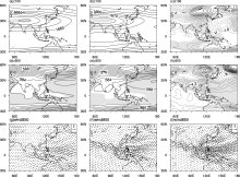
Figure 4 shows the composite geopotential heights at 100 and 500 hPa, and wind vectors at 850 hPa. In the upper troposphere (~100 hPa; Figs. 4a-c), the South Asia High (SAH) is weakened and shifted westward during the higher index years, but intensified and expanded longitudinally in the lower index years. For the 500 hPa geopotential heights (Figs. 4e and 4f), higher SSH_WCTP index is associated with a weakened and southward-shifted Western Pacific Subtropical High (WPSH), but is intensified and shifted to the west in lower index years. Besides, during higher index years there are cyclonic anomalies from East China to the midlatitudinal western Pacific. Northerly anomalies prevail over the southern coast of China, indicating a weakened EASM. Opposite changes are seen for lower index years. Nonetheless, higher (lower) SSHA_WTCP years are connected with a weakened (enhanced) EASM. These changes are even reflected clearly in their composite differences.
Previous studies have suggested that the interannual variability of the SSHA over the tropical Pacific is strongly connected with ENSO (Zhao et al., 2012). As shown in Fig. 2, the SSHA_WCTP index and simultaneous Niñ o 3.4 index have a high negative correlation of approximately -0.86, indicating that the two indices are not independent. While El Niñ o (La Niñ a) events occur in the preceding winter, the JFM SSHA over the WCTP region descends (ascends). Such an association is consistent with ENSO’ s connection with following-summer rainfall in China. However, comparing Figs. 3a and 3b, one can see more stations with significant rainfall correlation when the SSHA_WCTP index is used than when the Niñ o 3.4 index is used. This suggests that the SSHA_WCTP during JFM is more strongly connected with following-summer rainfall than ENSO. Thus, the SSHA_WCTP can be considered as a more effective predictor for summer rainfall than the Niñ o 3.4 index. 5 Conclusion and discussion In this study, we first investigate the associations of the preceding SSHA and SSTA with the following-fall IOD mode. The results suggest that the correlation of SSHA is higher than SSTA. Thus, an SSHA index is defined as the averaged SSHA over the WCTP and is referred to as the SSHA_WCTP. The preceding SSHA_WCTP index is positively correlated with the IOD, with the highest value of 0.46 occurring when the SSHA_WCTP leads the IOD by nine months.
The connection between the winter (JFM(0)) SSH index and following-summer rainfall in China is then investigated. The results suggest more rainfall in southern coastal China, along with less rainfall in the middle-lower reaches of Yangtze River, North China, and the Xinjiang region of Northwest China during higher index years. An overall opposite pattern is seen during lower index years. These features are in agreement with East Asian monsoon circulation anomalies. During higher index years, the WPSH is weakened, extends to the west and moves to the south. The SAH is weakened. Besides, northerly anomalies prevail over the southern region of China, which result in less water vapor transport to the Yangtze River valley and North China.
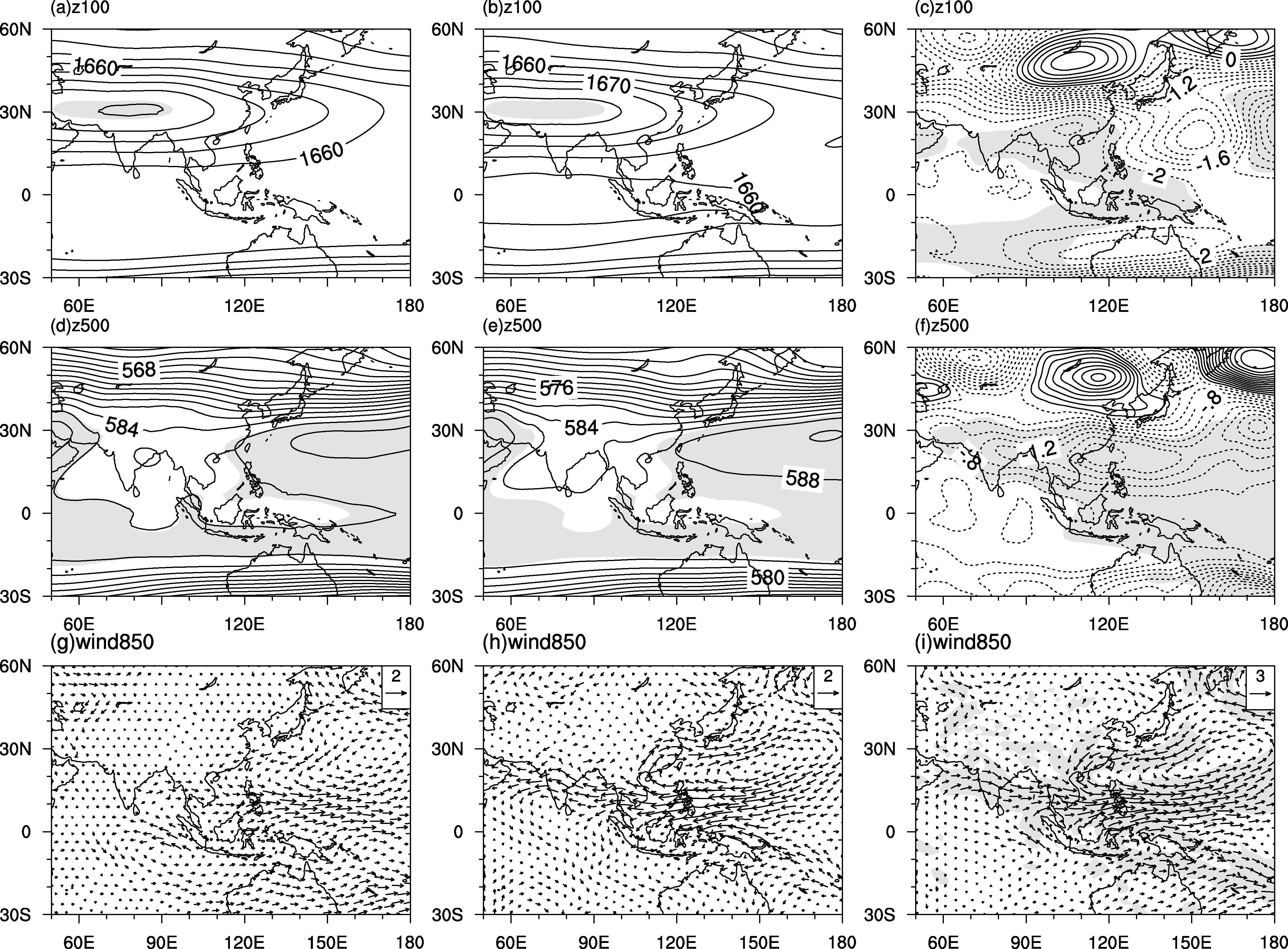 | Figure 4 Composite of the geopotential heights at (a-c) 100 hPa and (d-f) 500 hPa (gpdm), and (g-i) wind anomalies at 850 hPa (m s-1) for (left column) the higher index, (middle column) the lower index, and (right column) their difference. Shading areas in (a, b) and (d, e) denote the climatological location of the South Asia high and the western Pacific subtropical high, respectively. Shading in (c, f, i) represents significance above the 95% confidence level. The contour interval in (a, b), (d, e), and (c, f) is 5.0, 2.0, and 0.2, respectively. |
Zhao et al. (2012) revealed that the interannual variability of the SSHA over the tropical Pacific is related to ENSO development in certain months. The SSHA over the West Pacific descends when an El Niñ o event occurs. Here, we find that the SSHA_WCTP index has a significant negative correlation with Niñ o 3.4 index (approximately -0.86). Furthermore, we compare the correlations of summer rainfall with the SSHA_WCTP index and with the Niñ o 3.4 index and find that the former is more significant. Thus, the SSHA_WCTP index can be a more effective predictor for summer rainfall in China than the Niñ o 3.4 index.
Essentially, the SSHA reflects the subsurface thermohaline structure. Thus, regional-scale SSH anomalies may reflect both Rossby wave and local Ekman pumping dynamical processes earlier than the SSTA (Rao et al., 2010; Qiu and Chen, 2006). This seems reasonable because the SSTA reflects seawater thermodynamical responses, which take place much later than pure dynamical responses. Thus, the present finding that the preceding-winter SSHA leads the IOD more significantly than the SSTA may be realistic.
Furthermore, the interannual variations of the SSHA over the tropical Pacific Ocean may affect the strength of ITF transport. The connections between the SSHA over the WCTP region and the IOD may take place via the ITF. Then, the warm water transport from the tropical equatorial Pacific Ocean will lead to variations in thermocline and subsurface temperature anomalies over the Indian Ocean (Song et al., 2004; Yuan et al., 2011). It also suggests that the connections may arise from the propagation of ocean waves (Aparna et al., 2012; Sreenivas et al., 2012). The Rossby wave over the Pacific Ocean can propagate into the tropical Indian Ocean through the Banda Sea (Wijffels and Meyers, 2004). However, all the speculation still needs to be validated with numerical experiments using ocean-atmosphere coupled models. Thus, a more in-depth study is still required to explore the underlying physical mechanism.
The GODAS dataset used here only covers the period after 1980. This may be insufficient for the present study. To verify this, we use a much longer dataset from Simple Ocean Data Assimilation (SODAS), which covers the period 1958 to 2008, and conduct a similar analysis. The results suggest that the SSH signals over the WCTP region leading the IOD and summer rainfall are still there, albeit somewhat weakened (not shown). This suggests a robustness of the present finding. Finally, the SSHA- summer-rainfall connections are explained through its impacts on atmospheric circulation. The link between summer rainfall and the oceanic bridge is unclear, which also deserves further investigation.
| [1] |
|
| [2] |
|
| [3] |
|
| [4] |
|
| [5] |
|
| [6] |
|
| [7] |
|
| [8] |
|
| [9] |
|
| [10] |
|
| [11] |
|
| [12] |
|
| [13] |
|
| [14] |
|
| [15] |
|
| [16] |
|
| [17] |
|
| [18] |
|
| [19] |
|
| [20] |
|
| [21] |
|
| [22] |
|
| [23] |
|
| [24] |
|
| [25] |
|
| [26] |
|
| [27] |
|