An OGCM with a horizontal grid distance of less than (1/10)° is called an eddy-resolving OGCM, because it directly represents mesoscale eddies in most regions of the global ocean. An eddy-resolving OGCM can better capture the complex topography of the sea floor and the land-sea distribution. In addition, it can better describe the western boundary currents and other narrow currents. Consequently, it is important to develop eddy-resolving OGCMs, to better understand oceanic dynamics, as well their effects on climate change.

Eddy-resolving OGCMs have been widely used to investigate mesoscale eddies and the corresponding effects on climate in the North Atlantic basin (Smith et al., 2000; Oschlies, 2002). To date, several studies have diagnosed the ability of global eddy-resolving models in reproducing mesoscale eddies (Shriver et al., 2007; Thoppil et al., 2011). However, simulations of equatorial Pacific temperature and currents associated with ENSO in eddy-resolving OGCMs have rarely been analyzed in detail. In particular, we do not know how increased model resolution improves ENSO simulation. Meanwhile, despite being forced with observed wind stress and heat flux, many coarse resolution OGCMs exhibit very good performance in reproducing some basic ENSO characteristics, but few studies have explored the dynamic feedbacks in these models.

In the ocean-atmosphere system of the Pacific, many studies have used the Bjerknes index to evaluate the simulation ability of ENSO (Kim and Jin, 2011a, b). In particular, there are five linear feedback processes associated with the Bjerknes index: zonal advection feedback, thermocline feedback, Ekman feedback, mean advection feedback, and thermodynamic feedback. Thermocline feedback is the advection of anomalous temperature by mean vertical current, while Ekman feedback is the advection of mean temperature by anomalous vertical current. In the present study, we use the observed wind stress to force two versions of an ocean model. Thus, the ocean dynamic feedbacks are mainly discussed in this paper. The zonal advection feedback, thermocline feedback, and also the Ekman feedback play a positive role. However, the mean advection feedback and thermodynamic feedback have a damping effect on the Bjerknes index. Each feedback depends on the climatological mean state as well as the responses of the ocean (atmosphere) to the atmosphere (ocean). The present study analyzes the above important linear feedback processes related to ENSO.

The present paper attempts to answer two important questions: Does the simulation of equatorial Pacific temperature and currents improve as the model resolution is increased? And if so, what internal mechanism is for the impr responsible ovement?

The low resolution model (hereafter referred to as LICOM_L) is the LASG/IAP (State Key Laboratory of Numerical Modeling for Atmospheric Sciences and Geophysical Fluid Dynamics/Institute of Atmospheric Physics) Climate System Ocean Model, version 2 (LICOM2.0), which has been widely applied in many studies (e.g., Yu et al., 2011; Liu et al., 2012). The model is built using an Arakawa B grid. In particular, its dynamical framework is based on a latitude-longitude grid system with a 1° × 1° horizontal resolution. However, the meridional resolution between 10° S and 10° N increases from 1° to 0.5° , to better resolve the equatorial waveguide with an acceptable computational cost. The grid distance between 10° and 20° varies gradually from 0.5° to 1° . In addition, there are 30 layers with 15 equal-depth levels in the upper 150 m. The model is configured with realistic topography, except that the North Pole is set up as an isolated island. More details can be found in Liu et al. (2012).

The high resolution model (hereafter referred to as LICOM_H) is a quasi-global eddy-resolving OGCM based on LICOM2.0 but with many updates. For instance, the horizontal resolution is higher, at (1/10)° compared to 1° in LICOM2.0; there are more vertical layers (55, compared to 30), the thickness of the first layer is 5 m, there are 36 uneven layers in the upper 300 m, and thus the mean thickness is less than 10 m; and the model domain of LIOCM_H covers 66° N-79° S, meaning the Arctic Ocean is excluded. More details can be found in Yu et al. (2012). In addition, LICOM_H can simulate the observed meridional overturning circulation and meridional heat transport well (Mo and Yu, 2012). The performance regarding the representation of the Indonesian Throughflow, especially the mean vertical structures of the along-strait velocities, is improved in LICOM_H (Feng et al., 2013). Moreover, the outputs from LICOM_H have been successfully used to analyze the deep circulations of the South China Sea (Xie et al., 2013), as well as the eddy energy sources and sinks (Yang et al., 2013). Based on the control experiments in Yu et al. (2012), H. L. Liu (2012, personal communication) recently carried out longer term simulations with the two versions of LICOM (LICOM_H and LICOM_L) and using the same datasets from the Coordinated Ocean-Ice Reference Experiments (Large and Yeager, 2004) for the period 1948-2007. The model data used in the present study are for the period January 1958 to December 2001.

The ocean reanalysis data from the Simple Ocean Data Assimilation (SODA) (Carton and Giese, 2008) are compared with the model simulations. The ocean model of SODA has a horizontal resolution of 0.5° × 0.5° and 40 vertical levels. The monthly dataset used in this study is that of temperature from SODA2.0.2. The climatology fields are defined as the average over the period 1958-2001.

Climatological mean temperature in the equatorial upper ocean averaged over the whole 44 years from SODA, LICOM_H, and LICOM_L are shown in Fig. 1. These plots demonstrate that both LICOM_H and LICOM_L can capture the basic structure of the observed temperature, including the depth and zonal tilt of the equatorial thermocline, which is deeper in the west and shallower in the east. However, some discrepancies nevertheless exist, as indicated by the contours, which represent the temperature differences between the model simulations and reanalysis data. It is important to note that the simulated temperature in LICOM_H coincides well with the reanalysis in the eastern equatorial Pacific, especially the region between 100° W and 80° W, but there is an excessive warm bias in this region in LICOM_L. This illustrates that LICOM_H has a better simulation ability than LICOM_L in the eastern basin. In the western equatorial Pacific, both models demonstrate simulation bias. Moreover, it is important to note that the temperature bias in the off-equator region is more obvious than that at the equator (not shown). Thus, the temperature bias in the western equatorial Pacific could be mostly a result of the simulation in the off-equator region— an idea that will be analyzed in a future study. The present study pays attention to the simulation improvement in the eastern equatorial Pacific in LICOM_H.

Figure 1

	Figure Option ViewDownloadNew Window
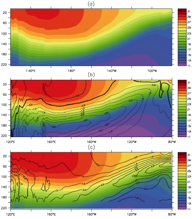	Figure 1 Time-mean temperature (color scale) in the equatorial upper ocean (5° N-5° S) in (a) Simple Ocean Data Assimilation (SODA), (b) High Resolution Model, and Low Resolution Model, and the corresponding temperature differences (contours) between (b) High Resolution Model and SODA and (c) Low Resolution Model and SODA. Units: ° C.

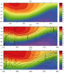
So, why are the temperature biases much improved in the eastern Pacific in LICOM_H? Because of the identical wind stress forcing used in the two models, the response of temperature to winds must be due to dynamic processes associated with the different spatial resolutions. Figure 2 presents the spatial pattern of temperature standard deviation in the equatorial upper ocean (color scale). In the eastern Pacific, the maximum temperature standard deviation is 2.4° C in the reanalysis and 2.4° C in LICOM_H, but 1.6° C in LICOM_L. This illustrates that the standard deviation in LICOM_H is more reasonable, which confirms again the significant improvement in the eastern ocean in LICOM_H. However, some biases also exist. The value of temperature standard deviation in the central Pacific is 2.8° C, which is a bit larger than that in the reanalysis (2.4° C). For the western Pacific, the standard deviation in LICOM_H around 160° E is larger than the reanalysis too. The overestimated standard deviation in LIOCM_H in the western Pacific may be attributable to the same cause of the bias in the mean state, mentioned above. Meanwhile, the contours in Fig. 2 present the regression coefficients of the temperature anomaly to the zonal wind stress anomaly in SODA, LICOM_H, and LICOM_L. The largest positive regression coefficient is 200° C (N m^-2)^-1 located at (60 m, 110-100° W) in SODA, 180° C (N m^-2)^-1 located at (60 m, 120-100° W) in LICOM_H, and 120° C (N m^-2)^-1 located at (60 m, 100-80° W) in LICOM_L. Both the strength and location of the maximum regression in LICOM_H are very similar to those in the reanalysis. This implies that the response of temperature to wind in the eastern equatorial Pacific is weaker in LICOM_L. It is worth noting that the largest negative coefficient in LICOM_H, located at (150 m, 160° E), is larger than in the reanalysis. This is due to the shallower mean thermocline in the western equatorial Pacific in LICOM_H, which would cause a more sensitive response of temperature to the wind stress anomaly. Although a certain degree of bias exists in the western basin, the simulated regression of temperature on wind in the eastern equatorial Pacific in LICOM_H is mostly close that in the reanalysis. This finding is manifested in the simulation improvement in the east, which is in line with the results shown in Fig. 1.

Figure 2

	Figure Option ViewDownloadNew Window
	Figure 2 The temperature standard deviation (color scale) in the equatorial upper ocean (5° N-5° S) in (a) SODA, (b) High Resolution Model, and (c) Low Resolution Model (units: ° C). The coefficients (contours) denote the response of the temperature anomaly (in 5° N-5° S) to the zonal wind stress anomaly (in (5° N-5° S, 120° E-90° W)) (units: ° C (N m-2)-1).

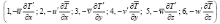
To better understand why the subsurface temperature anomalies are much improved in LICOM_H, we conduct a heat budget analysis using monthly mean temperature and currents in the region (0-100 m, (150-90° W, 5° N- 5° S)), where the maximum variability of temperature is observed. We base the analysis on the following temperature equation, as suggested by An and Jin (2004), for describing the heat budget of the ocean subsurface layer, in which the heat flux and subgrid-scale contributions (e.g., small-scale oceanic diffusion, heat flux due to tropical instability waves) are attributed to the residual term :

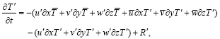
where the overbar denotes long-term mean temperature ( ) and velocity ( ), and the prime denotes the anomaly relative to the mean state. The first set of brackets includes the linear advection terms, while the second set presents the non-linear terms. The present study focuses mainly on linear advection. Figure 3 shows the heat budget results, in which the selected El Niñ o years (1965, 1972, 1976, 1982, 1986, 1991, and 1997) are the seven warmest years in the Niñ o3 region averaged in December to February (DJF) and, likewise, the chosen La Niñ a years (1970, 1973, 1975, 1984, 1988, 1998, and 1999) are the seven coldest years. In this way, we have the same number of events for both types, meaning the analysis is more reasonable and reliable. In addition, the data in the ENSO developing phase (from June to December) are used for the analysis. The plots demonstrate that the most important terms are - , - , and - . The term - reflects the effect of zonal advection feedback (Jin and An, 1999). Furthermore, the contribution of the vertical advection of temperature, - and - (representative of the thermocline and Ekman feedback, respectively), is in line with many previous studies (Jin, 1997; Jin and An, 1999; Huang et al., 2012). It is clear that the terms - and - possess the most significant differences between LICOM_H and LICOM_L, and thus both play an important role in inducing the simulation improvement in the eastern equatorial Pacific. The physical mechanism involved is described below.

Figure 3

	Figure Option ViewDownloadNew Window
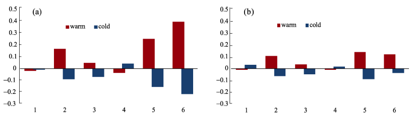	Figure 3 Heat budget analysis 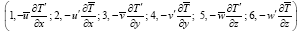averaged over the Niñ o3 region (5° N-5° S, 150-90° W) in the upper ocean (0-100 m) for the warm phase (red) and cold phase (blue) in (a) High Resolution Model and (b) Low Resolution Model. Units: ° C/month.

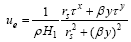
As discussed above, the vertical advection terms of - and - are the key factors in the improved simulation of ENSO. Furthermore, in the upper ocean, in LICOM_H is closer to the observation than that in LICOM_L, due to the increased vertical resolution— clearly seen in the results presented in Figs. 1 and 2. Thus, the differences of w′ and between LICOM_H and LICOM_L need to be detected in detail. Given the fact that the currents dataset in SODA suffers from some severe biases, we use an empirical formula to diagnose the zonal and meridional velocity, and then calculate w′ and . The anomalous Ekman currents are calculated based on Chang and Philander (1994), using

and

,

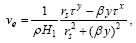
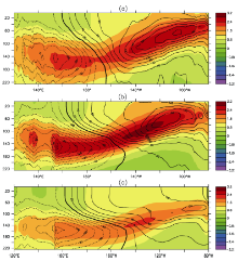
where β is the planetary vorticity gradient, ρ is the density of seawater; H₁ is the mean mixed-layer depth (here, we use 50 m); τ ^x and τ ^y are the zonal and meridional wind stress anomalies, respectively; and r_s = 0.5 d^-1 is the dissipation rate (Su et al., 2010). Figure 4 exhibits the anomalous Ekman currents, together with the w′ averaged over the Niñ o3 region simulated in LICOM_H and LICOM_L. The results show that the temporal evolution and magnitude of w′ in LICOM_H are more similar to the anomalous Ekman currents than they are in LICOM_L. This means that LICOM_H simulates a more reasonable w′ than LICOM_L, which could contribute to the Ekman feedback.

Figure 4

	Figure Option ViewDownloadNew Window
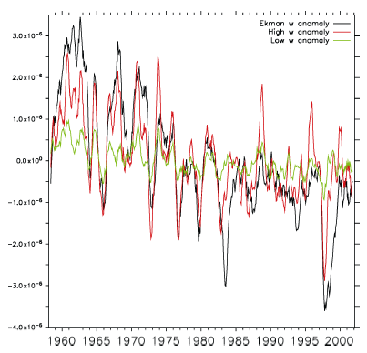	Figure 4 The anomalies of Ekman vertical currents (black line), the anomalies of vertical currents in High Resolution Model (red line), and the anomalies of vertical currents in Low-Resolution Model (green line), averaged over the Niñ o3 region (5° N-5° S, 150-90° W) in the upper ocean (0-50 m). Units: m s-1.

Keeping the other parameters as they are in Fig. 4, we replace τ ^x and τ ^y with monthly-mean wind stress in the above equation to obtain the monthly-mean vertical velocity. Figure 5 plots the simulated in LICOM_H and LICOM_L in comparison with the climatological mean Ekman current. A double-peak pattern exists in LICOM_H, which is identical to the mean Ekman current. Furthermore, the magnitude of in LICOM_H is more reasonable according to the three time series. Therefore, the improved simulation of in LICOM_H could also result in the improved thermocline feedback. In addition, the strengthened climatological mean upwelling is associated with the improvement in the climatological mean thermocline, and thus the more reasonable also contributes to the Ekman feedback. Besides their different spatial resolutions, it is necessary to emphasize two other main differences between LICOM_H and LICOM_L: the horizontal viscosity coefficient is different in the two versions of LICOM, and the parameterization of mesoscale eddies (Gent and McWilliams, 1990) is turned off in the equations of tracers in LICOM_H. Considering the above findings, the weakened horizontal viscosity coefficient is the key reason, as it results in stronger horizontal and vertical currents.

Figure 5

	Figure Option ViewDownloadNew Window
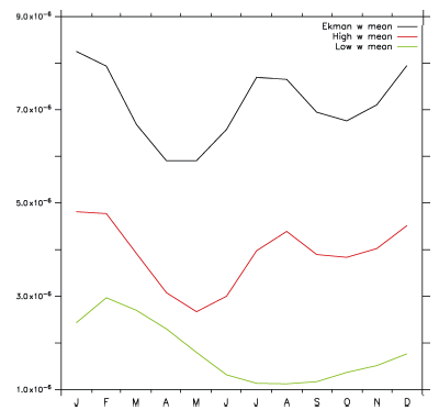	Figure 5 The monthly-mean vertical currents (black line), the monthly-mean vertical currents in High Resolution Model (red line), and the monthly-mean vertical currents in Low-Resolution Model (green line), averaged over the Niñ o3 region (5° N-5° S, 150-90° W) in the upper ocean (0-50 m) (units: m s-1).

Because the simulation of the equatorial Pacific temperature and currents associated with ENSO in LICOM_H has rarely been explored in previous studies, we conduct two numerical experiments, one using LICOM_H and one using LICOM_L, to help understand how the finer resolution of LICOM_H helps to improve the simulation of ENSO. Our main findings can be summarized as follows:

(1) The finer resolution improves the simulation of the mean state of, for example, the vertical temperature gradient in the upper ocean. Also, the vertical velocity near the surface is comparable with the Ekman current estimated from the observed wind stress.

(2) The vertical advections of temperature in the temperature equation are improved due to the contributions of both temperature gradient and velocity.

(3) Through heat budget analysis, the differences in vertical advections are much greater than those of zonal and meridional advection between LICOM_H and LICOM_L. This is manifested in the key roles played by the thermocline feedback and Ekman feedback in causing the amplitude of ENSO.

(4) Although the external wind stress forcing is exactly the same in the LICOM_H and LICOM_L experiments, the regression of temperature on wind stress is better reproduced in LICOM_H compared to that in LICOM_L, due to the above-mentioned more reasonable ENSO feedbacks.

It is important to acknowledge that there are some other details related to the high resolution of the model that need be further investigated in future studies. For instance, the role of nonlinear temperature advections, vertical mixing, and the effect of tropical instability waves are not considered in the present study. In addition, an attempt should be made to better understand the temperature bias in the western equatorial Pacific in LICOM_H.