To exemplify how the historical sampling approach works for ensemble-based data assimilation schemes, a brief introduction to DRP-4DVar is given first.

DRP-4DVar is one of the representative 4D ensemble-variational assimilation schemes (Wang et al., 2010). In DRP-4DVar, we first need to prepare the perturbed model space ensemble P_x and its projection onto the observation space, as follows:

To exemplify how the historical sampling approach works for ensemble-based data assimilation schemes, a brief introduction to DRP-4DVar is given first.

DRP-4DVar is one of the representative 4D ensemble-variational assimilation schemes (Wang et al., 2010). In DRP-4DVar, we first need to prepare the perturbed model space ensemble P_x and its projection onto the observation space, as follows:

(1)

(2)

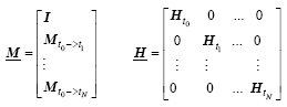
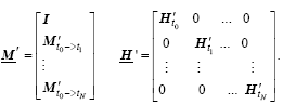
where x_b is the background and s is the ensemble size. Each member (column) of P_x represents the 3D model state increment (relative to the background x_b) in the beginning of the assimilation window, while each member (column) of P_Y represents the simulated observation increment (relative to the background simulated observation Y_b=Y(x_b)) within the whole window. Y(x), ‘ the observation simulator’ , consists of the forecast model and the observation operator, i.e., , while the operatorY’ (x’ ) is for simulating the observation increment, defined as:

(3)

The underlined letters represent 4D operators that are constructed by combining the 3D operators as

(4)

The letter I represents the unit matrix. The operator is the nonlinear model, integrating from t₀ (the beginning of the window) to t_i. is the observation operator at t_i, while and are their tangent linear operators, respectively.

As shown in Eq. (3), an approximate linear relationship between P_x and P_Y exists; thus, for the model space increment expressed as

(5)

its simulated observation increment is approximated linearly in the vicinity of x_b as

, (6)

where is the vector of linear combination coefficients.

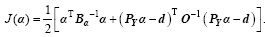
Thus, x’ and Y’ (x’ ) are replaced by linear operators (P_xa, P_ya, respectively). In this way, the DRP-4DVar cost function is an explicit quadratic function of a, as follows:

(7)

In Eq. (7), B_ais the BEC matrix with respect to a, O is the observation error covariance, and d is the innovation (observation minus background simulated observation). From the brief review above, the ensemble not only estimates the BEC, but also approximates Y’ (x’ ). So, it is inferred that the quality of the ensemble (P_x, P_Y) is crucial to the performance of DRP-4DVar. A simple flowchart of DRP-4DVar is given in Fig. 1a.

Note that in this work, for simplicity, we assume that the analysis time is in the beginning of the window; however, it can be tuned within the whole window for DRP-4DVar, as well as many other 4D ensemble-based methods (Liu et al., 2009; Zhao et al., 2011; Wang et al., 2011). Readers are referred to Wang et al. (2010) and Shen et al. (2014) for the detailed derivation of DRP- 4DVar.

Figure 1

	Figure Option ViewDownloadNew Window
	Figure 1 Flowcharts of (a) the Dimension-Reduced Projection 4DVar (DRP-4DVar), (b) the historical sampling process, and (c) the ensemble forecast sampling process.

As seen in the last section, DRP-4DVar, as well as many other ensemble-based schemes, needs to prepare the ensemble before minimization. Generally, an ensemble forecast is used to generate the ensemble at the analysis time by integrating the analysis ensemble of the last assimilation, i.e., through the ensemble cycling assimilation. Besides, for those 4D ensemble-based schemes that assimilate observations within the whole window, an extra ensemble forecast integration is needed to generate the observation space ensemble, i.e., Py=Y’ (Px). Thus, two ensemble forecast integrations are needed in each window. As a result, huge computational cost is expected.

The historical sampling approach is an alternative way to generate the ensemble much more efficiently. Wang et al. (2010) gave an example of how this sampling approach can be operated. In this example, two 78-h continuous forecasts with one output per hour are prepared, which are initialized with certain analysis data at 24 h and 48 h earlier than the beginning of the window, respectively. Figure 1b demonstrates the example of the sampling process for one historical series. Considering the assimilation window of 6 h, each 78-h forecast series contains 73 windows with each window shifted 1 h from another. So, 73 members are picked for each forecast series and a total of 146 members are obtained. As shown in Fig. 1b, the model space ensemble {x_i(t_o)} is obtained directly from the 1-h output of the model, while the observation space ensemble (the superscript h represents the ensemble generated by the historical sampling approach) is obtained by directly projecting the corresponding x_j(t_o) with the observation operators, i.e., for member index i (1≤ i≤ 73):

(8)

Thus, once the historical forecast series is prepared, no model integration is needed to generate the ensemble. Given the analysis-time background x_b and its projection on observation space Y_b, the perturbed ensemble members (i.e., members of P_x/P_Y) are calculated by subtracting the background from each member:

(9)

Although the historical sampling approach has many advantages, there is one potential problem associated with this method. As shown in Figs. 1b and 1c, unlike the ensemble forecast sampling approach, the integration intervals for historical ensemble members are shifted away from the assimilation window (00-06). As a result, the forcing (including sea surface temperature) and the lateral boundary condition (only for regional models) are different to that in the integration within the assimilation window. In fact, from Eq. (8), the underlying assumption for the historical sampling approach is that the prediction problem is an initial-value problem, where the forecast results are totally determined by the initial condition (IC). Besides, as the historical forecast series is a continuous run, the historical ensemble can be seen as generated by warm-start integrations, while in reality the ICs should be integrated in a cold-start way. As a consequence, these inaccurate integration configurations of the historical ensemble will probably introduce a special kind of sampling error for . For global models, which we are mainly concerned about here, the forcing difference and the ‘ cold-start or warm-start’ difference are the only two sources of the sampling error.

As shown in Fig. 1c, we can conduct an ensemble forecast in the correct configuration and initialized with the ensemble {x_i(t_o)} generated by the historical sampling approach. If the historical sampling approach has no such sampling error, its observation space ensemble should be the same as that integrated from the ensemble forecast (i.e., — the superscript f represents the ensemble generated by the ensemble forecast). Otherwise, the difference between and is exactly the sampling error. Thus, the integrated ensemble is a reference. In our evaluation experiment, GRAPES-GFS is adopted.

GRAPES-GFS (Zhang and Shen, 2008) is a global weather forecast system based on the GRAPES model, which is developed by the China Meteorological Administration. In this study, the GRAPES-GFS with a 1° resolution, 36 vertical levels, and 600-s time step configuration is utilized. Besides, the code is modified so that during the integration it outputs the input-file-formatted files every hour, which can be used directly as the initial input files for GRAPES-GFS.

Initialized with the 1° × 1° resolution National Centers for Environment Prediction final global tropospheric (NCEP/FNL) analysis, a 78-h integration starting from 0000 UTC 1 June 2011 provides a historical forecast series for the analysis at 0000 UTC 3 June 2011. Seventy-three ensemble members ({x_i(t_o)}) are picked, and then each is used as the IC to start a 6-h integration from 0000 UTC 3 June 2011, to generate the reference ensemble . The background x_b at 0000 UTC 3 June 2011 is obtained from the previous 6-h forecast, i.e., integrated from 1800 UTC 2 June 2011 and initialized with the NCEP/FNL analysis. Its projection onto observation space (Y_b) is obtained by integrating x_b within the assimilation window.

Here, it is assumed that the observations are measured directly on every grid point, so, in fact, no observation operators are performed. Furthermore, for additional simplicity, we assume the observations are at the end of the window. So, we just need to compare the terminal output of the model to begin with, but we then show the impact of the observations at different times at the end of section 3.2.

Using as the truth, we can measure the sampling error of by the global-averaged RMSE and correlation coefficient (CORR hereafter). Figure 2 shows the distributions of RMSE and CORR, along with the sampling time for six variables. As shown by the red (CORR) and blue (RMSE) solid lines, apparent diurnal cycle patterns exist for all of the six variables except surface pressure (Fig. 2b) and 500 hPa geopotential height (Fig. 2f), whose red lines are overlapped with the top border but the diurnal cycle patterns can still be observed if the figures are zoomed in. These diurnal cycle patterns can be attributed to the near diurnal variation of the radiance forcing. Among the six variables, skin temperature error has the largest amplitude, with its highest values of RMSE being over 6 K and its lowest values of CORR at around 0.96. This is because the land surface is heated directly by the downward radiance, and thus skin temperature is the most sensitive to the radiance. Furthermore, if we compare the remaining five variables, it is obvious that the thermal variables on lower levels, i.e., 850 hPa temperature (Fig. 2d) and 700 hPa humidity (Fig. 2e), have larger diurnal amplitudes than the other three variables. This is also evidence for the influence of the radiance forcing. We have also quantitatively estimated the contributions of the radiance forcing by calculating the empirical orthogonal function (EOF) decomposition of the sampling error along with the sampling time, and summing up the percentage variances explained by the spatial modes whose time series are significantly dominated by diurnal cycle patterns. For the variables corresponding to the subfigures in Fig. 2, the rates of contributions due to the radiance forcing are around 88%, 78%, 50%, 76%, 45%, and 92%, respectively. This suggests a dominant role played by the radiance forcing in the sampling error.

Figure 2

Figure Option ViewDownloadNew Window

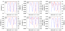
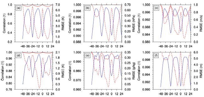Figure 2 Historical sampling error measured by global averaged RMSEs (blue lines) and correlation coefficients (red lines). The red solid lines represent the correlation coefficients of the original ensemble members (CORR), while the red dashed lines represent the correlation coefficients of the perturbed ensemble members (PCOR). Each figure represents one variable: (a) skin temperature; (b) surface pressure; (c) 925 hPa zonal wind; (d) 850 hPa temperature; (e) 700 hPa specific humidity; and (f) 500 hPa geopotential height. The horizontal axis represents sampling time (see Fig. 1b).

Besides the radiance forcing, the impact of the ‘ cold-start or warm-start’ integration difference can also be observed. From Figs. 2b-e, the -48-h shifted historical ensemble member has even smaller sampling errors than that of the 00-h shifted member. We speculate that the reason is that the -48-h shifted historical ensemble member is integrated in a ‘ cold-start’ configuration, the same as that of the reference, while the 00-h shifted historical ensemble member is integrated in the different ‘ warm- start’ configuration.

Although the evidence of the two sources of sampling error is clear, their magnitudes are very small, which suggests the 6-h integration can be approximated as an initial-value problem. However, it cannot be simply concluded that the historical sampling error is negligible. Actually, as shown in Eq. (7), it is the perturbed ensemble, rather than the original ensemble, that matters in the assimilation. So, we recalculate the correlation coefficients between the perturbed ensemble and the perturbed reference (PCOR hereafter) for further evaluation. As the large common component Y_b is subtracted from and , drastic decreases for PCOR over CORR, as shown by the red dashed lines in Fig. 2, are expected. Besides the decrease in values, the diurnal cycle patterns of PCOR are also disturbed. For all of the six variables, both the second and the third diurnal cycles ([-24, 0] and [0, 24] cycles) have larger amplitudes than the first cycle ([-48, -24] cycle). Let us use M(θ ; x) to denote the 6-h forecast operator, with θ denoting the forcing andx denoting the IC. Thus, if we perturb θ and x, we have the perturbed forecast as:

(10)

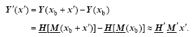
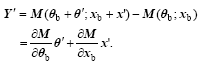
From Eq. (10), the perturbed forecast Y’ consists of two items, one caused by the perturbed forcing and the other caused by the perturbed IC . Furthermore, the smaller the magnitude of the perturbed IC (x’ ), the larger the proportion that the perturbed forcing (θ ’ ) contributes to the perturbed forecast (Y’ ). In extreme cases, where x’ is small enough, Y’ is totally determined byθ ’ , as follows:

(11)

For the historical ensemble members sampled during the second and third cycles, as their times are closer to the analysis time compared to the first cycle, they are more likely to have smaller perturbed ICs ( ), which we have verified already but the figures are omitted. As a result, the perturbed forcing contributes a larger proportion for the perturbed ensemble within the second and third cycles, and thus amplified PCORs of the second and third cycles are expected.

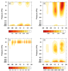
From the vertical distributions of the sampling error (PCOR shown in Fig. 3), besides the low level temperature, the stratospheric temperature is also perturbed in a diurnal cycle pattern, which can be attributed to the high concentration of ozone in the stratosphere. Influenced through the hydrostatic balance relationship, the high level geopotential height also shows a significant diurnal cycle pattern. For the specific humidity, many small- scaled large-negative-valued correlation noises exist above 100 hPa, especially around the 20 hPa level. However, we are unsure whether this small-scaled structure is model-dependent or physically reasonable. For the low level humidity (lower than 900 hPa), its sampling error also has a typical diurnal cycle pattern, with its minimum PCOR at around 0.8 (unrecognized in Fig. 3c). Unlike these three thermal variables, the zonal wind suffers only slightly from the sampling error.

Figure 3

	Figure Option ViewDownloadNew Window
	Figure 3 Vertical distributions of historical sampling errors (PCOR) for (a) temperature, (b) geopotential height, (c) specific humidity, and (d) zonal wind.

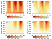
Until now, all the comparisons have been performed under the assumption that the observations are at the terminal end of the window. In Fig. 4, we give a simple demonstration of how the observation time influences the sampling errors. As expected, as the integration time increases, the forcing’ s contribution to the forecast results enlarges and the magnitudes of the sampling errors are amplified. These results suggest that the sampling error can be alleviated if a shorter assimilation window is selected or the analysis time is set in the middle of the window.

Figure 4

	Figure Option ViewDownloadNew Window
	Figure 4 Distributions of historical sampling errors (PCOR) along with the integrated time for (a) skin temperature, (b) 850 hPa temperature, (c) 20 hPa geopotential height, and (d) 925 hPa specific humidity.