
A New Scheme for Predicting Leaf Onset in Summer-Green Vegetation in the Northern Hemisphere
[TIAN Dong-Xiao1, 2 , ZENG Xiao-Dong1, *  ]
]
]
|
|


A modified thermal time model (MTM) was developed to reproduce the leaf onset for summer-green vegetation in the Northern Hemisphere. The model adopts the basic concept of a thermal time model (TM) in that leaf onset is primarily triggered by growing degree days (GDD). Based on global phenology data derived from satellite observations, a new parameterization for the critical model parameter Tb (i.e., baseline temperature for GDD calculation) has been introduced, and the spatial distribution of Tb was calculated. Simulations of leaf onset during 1982-2000 in the range 30-90°N showed a significant improvement of MTM over the standard TM model with constant Tb. The mean error and mean absolute error of the climatological simulation were 1.11 and 6.8 days, respectively, and 90% of the model error (5th and 95th percentiles) was between -12.4 and 13.7 days.
Leaf phenology is one of the most notable periodic plant phenomena that shapes the plant growth pattern, as well as the interaction between vegetation, climate, and environment. Changes in leaf area will directly influence carbon uptake and balance (Bachelet et al., 2001; Richardson et al., 2009; Feng et al., 2013; Keenan et al., 2014) and indirectly influence light competition among the plant community (Chuine et al., 2003). On the other hand, it also leads to changes in land-surface boundary conditions such as albedo and roughness, and hence has further impacts on the exchange of matter and energy between land and atmosphere (Pielke et al., 1998; Botta et al., 2000; Richardson et al., 2013).
Important leaf phenological events such as leaf onset and senescence depend primarily on climatic and environmental conditions including temperature, precipitation/soil moisture, and photoperiod (Richardson et al., 2013). For example, in temperate and boreal regions, warmth is the main controlling factor; deciduous plants usually shed their leaves during autumn and regrow their leaves during spring, and are thus referred to as summer-green plants. Ecological studies have shown that plants have developed a precise timing mechanism for leaf onset, in order to achieve the balance between avoiding damage by possible frost and pursuing greater carbon uptake (Adams, 2007).
Achieving a quantitative description of the correlation between leaf onset and climate factors is crucial for both ecological studies and climate modelling studies. The most direct and simplest approach is to use a temperature threshold as a criterion (Foley et al., 1996). Although this method can to a certain extent reproduce the multi-year averaged leaf onset date as a function of the climatology of daily temperature, large errors exist when it is applied to simulate the annual phenology, due to the large fluctuation of daily temperature in spring. To avoid such a problem, Cannell and Smith (1983) applied the concept of growing degree days (GDD) and developed the thermal time model (TM). Generally speaking, there are two critical parameters in the TM model: a baseline temperature for calculating GDD, and a GDD threshold for triggering leaf onset, which are usually constant or dependent on species only. However, various modelling studies (e.g., Richardson et al., 2012) have shown the deficiencies of such a simple parameterization scheme when applied at global or large scales.
In recent years, the rapid increase in global satellite observational data (including phenological data) have provided the possibility of better estimation of the critical parameters in the TM model. In this study, we developed a modified thermal time model (MTM) to predict the climatological and annual leaf onset date from 1982 to 2000 north of 30° N. In section 2, we introduce the study area, input dataset (including leaf onset data and temperature data). In section 3, we describe the MTM model, and in section 4 we report the simulation results for the climatological and annual leaf onset date. Finally, in section 5 we conclude our research with some discussion.
The study area covered 30-90° N, with a spatial resolution of 0.5° × 0.5° . Information on vegetation cover was obtained from the land surface data of the Community Land Model, version 4.5 (CLM4.5). We focused on the land area dominated by plant functional types (PFTs) with summer-green phenology, including broadleaf or needleleaf deciduous tree (temperate or boreal), broadleaf deciduous shrub (temperate or boreal), and C3 grass (arctic or non-arctic). The number of samples was 12 079, which was about 60.5% of the natural vegetation coverage.
The data on leaf onset used in this research were derived from a long-term Global Land Surface Satellite (GLASS) dataset (Liang et al., 2013). The GLASS products include leaf area index (LAI), broadband albedo, broadband emissivity, downward shortwave radiation, and photosynthetically active radiation. The LAI product is derived from Advanced Very High Resolution Radiometer (AVHRR) and Moderate Resolution Imaging Spectroradiometer (MODIS) ranging from 1982 to 2012. A modified piecewise logistic fitting method was utilized to derive leaf phenology from LAI (Zhang et al., 2003), and zero point of the forth order derivative of the fitted logistic models was used to determine the four transition dates, including green-up, maturity, senescence, and dormancy, for each phenology cycle (in these phenological data, there were up to two phenological cycles for each year).
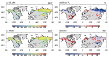
Since most natural vegetation has only one phenology cycle, only green-up in the first phenology cycle from 1982 to 2000 was used as the leaf onset date in this research. We also calculated its multi-year average to obtain the climatology of leaf onset, which we named Phe8200. The spatial distribution of Phe8200 is shown in Fig. 1a.
 | Figure 1 (a) Spatial distribution of leaf onset dates for summer-green plants in Global Land Surface Satellite (GLASS) dataset (b) Fitted Tb; (c) Simulated leaf onset date in Experiment 1 (EX1); (d) The difference between model and observation. |
We utilized a global land surface air temperature (SAT) dataset produced by Wang and Zeng (2013), which was developed from four reanalysis products: Modern-Era Retrospective Analysis for Research and Applications (MERRA), for 1979-2009; 40-yr European Centre for Medium-Range Weather Forecasts (ECMWF) Reanalysis (ERA-40), for 1958-2001; ECMWF Interim Reanalysis (ERA-Interim), for 1979-2009; and National Centers for Environmental Prediction-National Center for Atmospheric Research (NCEP-NCAR) reanalysis, for 1948-2009. Climatic Research Unit (CRU) monthly-mean maximum and minimum data were applied for bias correction. Wang and Zeng (2013) showed that this dataset performed well, in comparison with in-situ hourly measurements, over six sites and with a regional daily SAT dataset over Europe; hence, it could provide better estimation of daily mean temperature.
The spatial resolution of the original dataset was 0.5° × 0.5° , and the temporal resolution was one hour. We aggregated the data into daily temperature. The climatology from 1982 to 2000 was calculated and named Tem8200.
The TM is a mechanistic model developed by Cannell and Smith (1983). It is based on known or assumed cause-effect relationships between biological processes and environmental driving factors (Chuine et al., 2003). The TM is described by GDD, which is defined as
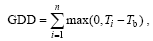 (1)
(1)
where i is the day of year, Ti is the temperature of the ith day, and Tb is the baseline temperature. In some applications, e.g., CLM-DGVM (dynamic global vegetation model) 3.0 (Levis et al., 2004), GDD is reset to 0 when Ti< Tb, an approach used to avoid the influence of cold injury. Plants start leaf shooting until GDD exceeds a preset critical value (Vc).
Due to the lack of large-scale phenological observations during the early development of the TM, Tb was preset as a global constant or a parameter depending only on species, biomes or PFTs. Although in different applications Tb may have different preset values, they have no spatial or temporal variation.
The TM has been introduced into DGVM; for instance, CLM-DGVM 3.0 (Levis et al., 2004), CLM-CNDV 4.5 (Bonan et al., 2013), SEIB (spatially explicit individual-based dynamic global vegetation model)-DGVM (Sato et al., 2007), and IAP-DGVM (Zeng et al., 2014). Such simplification, however, has caused large errors when applied at global or large scales (Richardson et al., 2012). For example, as GLASS phenology data were analyzed in the present study, the temperature on leaf onset dates in northern Canada, Russia, and Europe was below 0° C, much lower than in temperate regions. Hence, if Tb was set to 0° C for the whole study area, it was not surprising that the model predicted a systematic delay in leaf onset, increasing with latitude (see section 4.2 and Fig. 2b for more information).
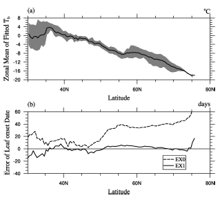 | Figure 2 (a) The zonal mean of model Tb, shaded area is between the 25th and 75th percentile of model Tb; (b) The error of the zonal mean in the control Experiment (EX0) (dash line) and EX1 (solid line). |
Regarding the dramatic geographical range of the distribution of summer-green vegetation, it is reasonable to assume that both Tb and Vc vary with location. Actually, the value of Tb has been assigned within a wide range in previous studies. For instance, Hunter and Lechowicz (1992) selected -5° C, 5° C, and 15° C for 26 species of native hardwood trees in Ohio, and Botta et al. (2000) chose -5° C, 0° C, and 5° C for different boreal/temperate biomes. In this study, we developed an MTM in which Tb was estimated from global phenological observations and local climate conditions.
Technically speaking, the spatial distribution of Tb can be inferred from satellite-observed global phenological data (and hence is called “ observed” Tb). By applying GLASS phenological data and the temperature data of Wang and Zeng (2013), and setting Vc to be 100, the value of Tb can be calculated using Eq. (1), by employing the method of dichotomies to search between the temperatures on 1 January and leaf onset date, and controlling the error of GDD below 0.5. However, such a method might not be of practical use in climate models and DGVMs, because the errors in observations (especially in phenological data) may be amplified in plant phenology. Furthermore, it could not produce the historical variation of Tb, and hence may be inapplicable to studies of paleo- or future climate.
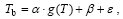
An alternative approach is to relate Tb with climate factors that are available in climate models. Our study indicated that there was a significant linear relationship between Tb and spring temperature g(T) (the average temperature from March to May), and the regression function can be written as:
 , (2)
, (2)
where α and β are fitted parameters, and ε is the residual error.
To obtain a robust result, the climatological data, i.e., Phe8200 and Tem8200, were used for the regression. We obtained α =0.72 and β =-4.50, while the residual standard error of the fitting was 0.0027, and the coefficient of determination R2 was 0.84. In the following analysis, we denote Tb simulated by Eq. (2) as Tb_mod. The average of Tb_mod throughout the study area was -8.1° C, ranging between -19.9° C and 11.5° C, with standard deviation of 5.7° C— roughly the same as the “ observed Tb” . Figure 1b shows the geographical structure ofTb_mod, and Fig. 2a shows that its zonal average decreased with latitude.
Three experiments were performed for model verification. In Experiment 1 (EX1) and Experiment 2 (EX2), Tb_mod was applied. While EX1 used Tem8200 to predict the climatology of leaf onset date and was compared with Phe8200, EX2 used temperature in each year from 1982 to 2000 to show the interannual variability of predicted phenology. The control experiment, EX0, had Tb_mod ? 0, which represented a standard TM scheme (the same as in IAP-DGVM and CLM-DGVM 3.0), and also Tem8200 to predict a climatology for comparison with EX1. In all experiments, the GDD requirement of Vc was 100.
For each experiment, the mean error (ME) and mean absolute error (MAE) of the simulated leaf onset date were calculated as follows:
 (3)
(3)
where n is the number of samples, xi is prediction, and yi is observation.
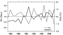
In order to evaluate the interannual variability, the error in the predicted climatology of leaf onset, i.e., EX1, should be removed from EX2. Thus, the anomaly of model error (denoted as EA) was calculated as follows:
EAj=MEj-MEcli, (4)
where j is the index of year, MEj is the mean model error in year j in EX2, and MEcli is the mean model error for Phe8200 in EX1. To further analyze EA, the climate interannual variability, i.e., the anomaly of spring temperature (denoted as STA), was also introduced as:
SATj=STj-STcli , (5)
where STj is the mean spring temperature in year j, and STcli is the mean spring temperature for the climatology of 1982-2000.
Figure 1c shows the spatial pattern of leaf onset simulated in EX1. The ME of EX1 was 1.11, and the MAE was 6.8 (days). The 5th, 25th, 75th, and 95th percentile values of the model error were -12.4, -3.1, 6.9, and 13.7 (days), respectively. The MTM captured the overall spatial pattern of leaf onset as in the observation (Fig. 1a), matched well in Russia, but the predicted leaf onset dates were later than observed in most of North America and Nordic Europe, and earlier in most of northern China (Fig. 1d). Figure 2 shows that the error of the zonal mean in EX1 was close to zero between 40° N and 75° N.
On the contrary, much larger errors existed in EX0, in which the ME was 31 and the MAE was 32.4 (days). The bias of the zonal mean was larger than 30 days between 50° N and 80° N (Fig. 2b), consistent with the region where Tb was much lower than 0° C (Fig. 2a). This shows the considerable advantage of a spatially variable Tb over a constant Tb in predicting leaf onset date.
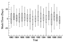
Figure 3 shows that model error varied for different years in EX2. For all 19 years, the average ME of EX2 was 1.87 and the average MAE was 10.6. For each year, the ME was between -3.1 and 7.16 and MAE was between 8.23 and 12.9. Sixty-one percent of model error fell in to the interval between -10 and 10 days, and 87.2% was between -20 and 20 days.
 | Figure 3 Box plot of model error from 1982 to 2000 in Experiment 2 (EX2). The bottom and top of the box are the first and third quartiles, the band inside the box is the median, and the ends of the whiskers are the 5th and 95th percentiles. |
Figure 4 shows that the anomaly of model error (EA) and the corresponding anomaly of spring temperature (STA) were to a certain extent correlated. The correlation coefficient between EA and STA was -0.623, significant at 0.01 level. Generally, EA was positive when spring temperature was cooler, and negative when spring temperature was warmer than climatology, i.e., the model overestimated the phenological shift induced by the temperature anomaly. This implies that, while plants may adapt to the local climate during their evolutionary history, they are less capable of adjusting to interannual climate variability or disturbance.
 | Figure 4 Anomaly of model error (denoted as EA, dash line) and anomaly of spring temperature (denoted as STA, solid line) from 1982 to 2000 in EX2. |
We developed an MTM to predict leaf onset for summer-green plants in the region of 30-90° N. The baseline temperature for GDD calculation, Tb, was calculated by a linear regression equation of spring temperature. Simulation results showed a significant improvement of the MTM over the standard TM with constant Tb. The ME and MAE of the climatological simulation was 1.11 and 6.8 days, respectively, and 90% of the model error (5th and 95th percentiles) was between -12.4 and 13.7 days. For the annual simulation from 1982 to 2000, the ME was 1.87 and the MAE was 10.6 days.
The MTM could be easily applied to large-scale models such as DGVMs, as long as the parameters of α and β are provided. Because Tb is calculated from spring temperature, there is no requirement to provide an extra dataset of Tb with different spatial resolutions. The values of α and β can be easily calibrated when longer term and better quality phenological data are available. The MTM could even be applied in studies of the paleo- or future climate by attributing the phenological shift to the changes in the climatology of spring temperature, although such an assumption needs further investigation.
The spatial variation of Tb may represent a plant’ s adaptive strategy in response to climate and environmental conditions. For example, both our study and results from MODIS (Zhang et al., 2006) show that the temperature on the leaf onset date is below 0° C over the boreal region, where plants are more acclimatized to cold temperature (Sakai and Larcher, 1987); hence, it is reasonable that Tb< 0° C. Of course, the linear correlation between Tb and spring temperature is only a primary approximation. The bias in the semi-arid region (30-35° N) and artic region (> 75° N) in Fig. 2b implies that other climate criteria, such as precipitation and photoperiod, should be taken into account.
| 1 |
|
| 2 |
|
| 3 |
|
| 4 |
|
| 5 |
|
| 6 |
|
| 7 |
|
| 8 |
|
| 9 |
|
| 10 |
|
| 11 |
|
| 12 |
|
| 13 |
|
| 14 |
|
| 15 |
|
| 16 |
|
| 17 |
|
| 18 |
|
| 19 |
|
| 20 |
|
| 21 |
|
| 22 |
|