ZHANG Hong-Qin, TIAN Xiang-Jun, ZHANG Cheng-Ming. An Economical Approach to Flow-Adaptive Moderation of Spurious Ensemble Correlations and Its Application in the Proper Orthogonal Decomposition-Based Ensemble Four Dimensional Variational Assimilation Method. Atmospheric and Oceanic Science Letters, 2015, 8(5): 320-325
Permissions
Copyright?2015, Editorial office of Atmospheric and Oceanic Science Letters
This is an Open Access article under the terms of CCAL.
An Economical Approach to Flow-Adaptive Moderation of Spurious Ensemble Correlations and Its Application in the Proper Orthogonal Decomposition-Based Ensemble Four Dimensional Variational Assimilation Method
1 Shandong Agricultural University ,College of Information Science and Engineering, Taian 271000, China 2 International Center for Climate and Environment Sciences, Institute of Atmospheric Physics, Chinese Academy of Sciences, Beijing 100029, China
The purpose of this study is to describe an economical approach to an existing adaptive localization technique and its implementation in the proper orthogonal decomposition-based ensemble four-dimensional variational assimilation method (PODEn4DVar). Owing to the applications of the sparse processing and EOF decomposition techniques, the computational costs of this proposed sparse flow-adaptive moderation (SFAM) localization scheme are significantly reduced. The effectiveness of PODEn4DVar with SFAM localization is demonstrated by using the Lorenz-96 model in comparison with the Smoothed ENsemble Correlations Raised to a Power (SENCORP) and static localization schemes, separately. The performance of PODEn4DVar with SFAM localization shows a moderate improvement over the schemes with SENCORP and static localization, with low computational costs under the imperfect model.
Data assimilation is an analysis technique in which the observed information is combined with forecasted information to estimate the states of a system. The background error covariance (B) plays an important role in data assimilation system. It is essential for several reasons, such as information spreading, information smoothing, balance properties, the ill-condition of the assimilation, and flow-dependent structure functions. In the standard four-dimensional variational assimilation method (4DVar) (e.g., Lewis and Derber, 1985; Le Dimet and Talagrand, 1986; Courtier and Talagrand, 1987; Courtier et al., 1994), we usually apply the background error covariance modes to produce an homogeneous and isotropic B. This method makes the background error covariance estimation much easier, but it is not always appropriate under some conditions. To improve the background error covariance estimation, using ensemble forecast statistics to produce B is a more attractive approach (e.g., Evensen, 1994). Ensemble-based data assimilation methods (e.g., Evensen, 1994; Qiu et al., 2007; Tian et al., 2008, 2011; Wang et al., 2010; Tian and Xie, 2012; Tian and Feng, 2015) have the ability to evolve flow-dependent estimates of forecast error covariance (i.e., the background error covariance B) by forecasting the statistical characteristics. However, the use of finite ensembles to approximate the error covariance inevitably introduces sampling errors that are seen as spurious correlations over long spatial distances. Such spurious correlations could be ameliorated through the localization process (e.g., Houtekamer and Mitchell, 2001; Hamill et al., 2001).
Localization is a useful strategy for reducing the effect of spurious ensemble correlations caused by small ensembles. Usually, localization acts by constructing a moderation function and representing B as a Schur product of the ensemble correlation function and moderation function. The most common method of constructing the moderation function for reducing the effect of spurious correlations is applying some types of distance-based functions (e.g., Houtekamer and Mitchell, 1998, 2001; Gaspari and Cohn, 1999; Hamill et al., 2001). Studies also show that different localization functions can be used for different observation types (Houtekamer and Mitchell, 2005; Tong and Xue, 2005; Lei and Anderson, 2014), and various state variables (Anderson, 2007, 2012). Although good results have been obtained, for large models, tuning the width of the localization coefficient can be expensive (e.g., Anderson and Lei, 2013). Furthermore, vertical localization has been more challenging, while many large ensemble filter applications have localized observation impact in the horizontal direction.
To address the aforementioned issues, there have been several methods proposed to construct the moderation function in a flow-adaptive way. The hierarchical approach in Anderson (2007) utilizes a Monte Carlo method based on splitting the ensemble into several small ensembles to assess the sampling errors and the spurious correlations. Zhou et al. (2008) introduced a multi-scale tree concept and it worked well, especially when the update calculations have the same structure as the tree. Emerick and Reynolds (2010) believed that the key point of the localization procedure is choosing the critical length(s), based on the model correlation length(s) and the range of the sensitivity matrices. Bishop and Hodyss (2007) proposed the Smoothed ENsemble Correlations Raised to a Power (SENCORP) approach based on the online computation of a low-dependent moderation function that damps long-range and spurious correlations. Numerical assimilation experiments demonstrate that SENCORP moderation functions are superior to non-adaptive moderation functions. Since many matrix products and eigenvector decompositions have to be performed in SENCORP, its computational costs are thus expensive. Furthermore, the SENCORP approach cannot be directly applied in the ensemble-based 4DVar methods (e.g., Tian et al., 2010; Wang et al., 2010) in which the spurious correlations between the model grids and observational sites should be ameliorated, since it can only provide moderation functions over the model grids.
This paper describes an economical approach to implement the SENCORP method and further enable it to be applied in the proper orthogonal decomposition-based ensemble 4DVar (PODEn4DVar) (Tian et al., 2010) through the EOF decomposition and interpolation technique. In section 2, we describe the SENCORP localization scheme and its modification version, named the sparse flow-adaptive moderation (SFAM) localization technique, proposed in this paper, and its implementation in the PODEn4DVar method. In section 3, observing system simulation experiments (OSSEs) are conducted using PODEn4DVar with the static localization, the original SENCORP moderation localization, and the newly proposed SFAM localization schemes, for evaluation of SFAM. Finally, a summary is given in section 4.
2 The SFAM scheme and its implementation in PODEn4DVar
2.1 SFAM localization
Bishop and Hodyss (2007) proposed the SENCORP algorithm to generate moderation functions from a smoothed covariance function, which damps small correlations when raised to a power. The construction of SENCORP moderation functions requires the following steps:
Step 1: Let X=[x1, x2, …, xK] be n× K ensemble samples, where K is the total sample number and n is the size of the model state vector. is the corresponding sample perturbations,
(1)
. (2)
The smoothed perturbations are thus obtained by applying a Gaussian filter to the original perturbations X’ with a smoothing parameter ds.
Step 2: The normalized spatiotemporally smoothed ensemble perturbations are further computed through , where is the jth variable of the ith smooth ensemble and .
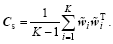
The sample correlation matrix Cs of the smoothed ensemble perturbations is thus obtained,
. (3)
Step 3: Give Cs power m to reduce small spurious correlations.
(4)
and
(5)
Step 4: The matrix product smoother is obtained by taking the matrix product of with itself q times to obtain and renormalizing this matrix through
(6)
where .
Step 5: The SENCORP moderation function is finally given by attenuation of the spurious correlations amplified by going from , i.e.,
, (7)
where r is the element-wise integer power.
For more details of the above process, please refer to Bishop and Hodyss (2007). The many matrix products and eigenvector decompositions involved in the SENCORP algorithm (i.e., steps 1-5) will certainly result in high computational costs. Furthermore, the SENCORP approach cannot be directly applied in the ensemble-based 4DVar methods (e.g., Tian et al., 2010; Wang et al., 2010) in which the spurious correlations between the model grids and observational sites should be ameliorated, since it can only provide moderation functions over the model grids.
To address the aforementioned issues, we firstly construct the SENCORP matrix CSENCORP on low-resolution (and thus sparse) grids, so that the computational cost is significantly reduced. That is, we firstly implement steps 1-5 to obtain a sparse (i.e., low-resolution) (ns is the size of the model state vector on the low-resolution grids), which is followed by its decomposition ( ) using EOF decomposition,
(8)
and
(9)
where E contains all of the eigenvectors, λ is a diagonal matrix whose diagonal elements are eigenvalues, and . Each line of the local correlation ensemble C’ corresponds to each element of the model states. Consequently, the local correlation ensemble C of the high-resolution grid could be obtained by spline interpolation from C'. Because a few eigenvectors can represent the correlation function very well, in actual implementation, we only utilize the first rcolumns of the local correlation ensemble C’ , and thus the computational cost of C (on the high-resolution grid) is greatly reduced.
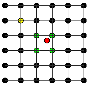
To implement the SFAM localization scheme in PODEn4DVar, we should further give the moderation correlations between each model grid and the observational locations, which can also be solved by a simple interpolation procedure. Figure 1 is a schematic diagram of such an interpolation procedure. Suppose that the red circle is one observation location, one can easily utilize the local correlation samples over its nearby model grids (for example the green grids) to interpolate the local correlation samples cy, j(j=1, …, l, where l is the number of measurements) for this observational location. Consequently, the moderation element (CSFAM)ij between the ith model grid and the jth measurement is computed by
Figure 1 Linear interpolation for correlations between model grids and observational grids (the red circle is one observation location, and the green and yellow circles are model grids).
2.2 The implementation of SFAM in PODEn4DVar
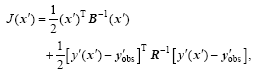
By minimizing the following incremental format of the 4DVar cost function, Eq. (11), one can obtain an optimal increment of the initial condition, , at the initial time,
(11)
where x’ =x-xb is the perturbation of the background field xb at the initial time t0,
(12)
(13)
(yk)’ =yk(xb+x’ )-yk(xb), (14)
y’ obs, k=yobs.k-yk(xb), (15)
yk=Hk(Mto?tk(x)), (16)
(17)
Here, the superscript T represents a transpose, b denotes the background value, the index k stands for observation time, S is the total observational time steps in the assimilation window, Hk acts as the observation operator, and the matrices B and Rk are the background and observational error covariance, respectively. One should minimize the 4DVar cost function, Eq. (11), to obtain an optimal increment of the initial condition, , at to.
With the prepared background field xb, the initial model perturbations , the simulated observation perturbations , the observational increments , and the background and observational error covariance B and Rk, the final PODEn4DVar analysis increment solution without localization is formulated through some necessary calculations (see Tian et al. (2011) for more details) as
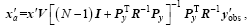
, (18)
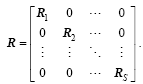
where V is an orthogonal matrix and is derivable from is a diagonal matrix, I is the unit matrix and Py=y’ V. To clarify, the background covariance B is approximately estimated by (Px=x’ V) in formulating PODEn4DVar.
We mark
(19)
and rewrite Eq. (18) as follows:
(20)
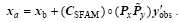
Similar to Tian et al. (2011) and Tian and Xie (2012), the SFAM function is applied to the matrix , and the final PODEn4DVar analysis is calculated using the formula
(21)
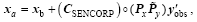
For comparison, we also implement the SENCORP and static localization schemes in to PODEn4DVar, as follows:
(22)
and
(23)
where each elementρ i, j (of the modification matrix ρ ) is given by Eqs. (31)-(32) in Tian and Feng (2015).
3 Evaluations within a Lorenz96 model
3.1 Experimental design
In this section, the PODEn4DVar approach with the SFAM scheme is evaluated within the model of Lorenz (1996),
(24)
with cyclic boundary conditions, x-1=xn-1, xo=xn, and xn+1=x1. One can choose any dimension, n, greater than 4 and obtain chaotic behavior for suitable values of the external forcing F. In this configuration, we take n = 40 and F = 8. Here, F = 8 represents the perfect model to produce the “ true” and “ observational” fields. However, in the following assimilation experiments, we adopt F = 9. For computational stability, a time step of 0.05 units (or the equivalent of 6 h in Lorenz (1996)) is applied. The experimental settings are completely the same as those described in Tian et al. (2011).
The performance of PODEn4DVar with the SFAM scheme is examined in comparison with the SENCORP localization scheme (Bishop and Hodyss, 2007) and the one with static localization (Tian et al., 2011). In the following experiments, we choose a low resolutions (e.g., only retaining one grid every two model grids) to construct the SFAM modification function to exploit an appropriate resolution. Also, we test the parameter sensitivity contained in the SFAM modification function, which is the function of m, q, r, and the smoothing parameter ds. The default number of observations is equal to 20 (equally spaced at every observation time). Observations are taken every two steps (or 12 h), generated by adding random error perturbations of 0.03 to the time series of the true state (F = 8). We consider an assimilation window length of 4 (standard 24-h daily assimilation cycle). The default parameter setups for the static localization scheme (only one direction in the Lorenz-96 model) are: ensemble size N = 60 and Schur radiusr0=4.
3.2 Experimental results
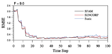
Figure 2 compares the performance of PODEn4DVar with the SFAM, SENCORP, and static localization techniques under the imperfect-model assumption (F = 9). It shows that all three techniques behave very well in terms of overall low root-mean-square error (RMSE). SFAM performs slightly better than the other techniques, especially in the first 20 time steps. The time steps are followed by their almost identical performance until the end of the whole assimilation process. The performance of SENCORP is similar to the static scheme. The performance of SFAM is superior to SENCORP, which is likely due to the application of EOF decomposition in SFAM. EOF decomposition can capture the main spatial correlation information of state variables and disregards some of the Gaussian white noise for better moderation.
Figure 2 Time steps of RMSEs for the three localization techniques (Sparse Flow-Adaptive Moderation (SFAM), Smoothed Ensemble Correlations Raised to a Power (SENCORP), and Static) using default parameter setups with the Lorenz-96 model with model error F = 9.
To examine the sensitivity of the PODEn4DVar assimilation to the variations of the parameters of the SFAM localization technique, we design four groups of experiments. Figure 3a shows that the smoothing parameter ds has slight impacts on the PODEn4DVar assimilation under the imperfect-model assumption. The performance of ds =16 is superior to any of the others. Figure 3b shows parameter m also has slight impacts on the PODEn4DVar assimilation under the imperfect-model assumption. Generally, we choose m= 2. Figure 3c shows the performance of the PODEn4DVar assimilation is sensitive to the variations of parameter q. When q= 2, the performance of the PODEn4DVar assimilation is stable and the RMSEs are the lowest. Figure 3d demonstrates that parameter r has slight impacts on the PODEn4DVar assimilation under the imperfect-model assumption. Parameter m has the same function as r; we also choose r = 2.
Figure 3 Time steps of RMSEs for different parameters of SFAM with the Lorenz-96 model with model error F = 9: (a) smoothing parameter ds; (b) m; (c) q; (d) r.
For the two groups of experiments, the ratio of the computational costs for the three (i.e., SFAM, SENCORP, and static) localization schemes is about 1:1.5:2.3. Thus, the SFAM scheme is efficient due to its sparse processing and EOF decomposition techniques.
4 Summary and concluding remarks
This study has proposed the SFAM localization technique and implemented it in PODEn4DVar. The robustness and potential merits of the implementation of PODEn4DVar with SFAM localization have been demonstrated by using the Lorenz-96 model. For comparison, the implementation of PODEn4DVar with the SENCORP localization and static localization have also been tested by using the Lorenz-96 model. The assimilation results imply that, to a certain extent, PODEn4DVar with SFAM localization outperforms PODEn4DVar with the SENCORP and static localization schemes. The computational costs of PODEn4DVar with SFAM localization are significantly more efficient than PODEn4DVar with SFAM localization due to its sparse processing and EOF decomposition techniques.
Reference
1
AndersonJ. L. , 2007: Exploring the need for localization in ensemble data assimilation using a hierarchical ensemble filter, Phys. D, 230, 99-111.
2
AndersonJ. L. , 2012: Localization and sampling error correction in ensemble Kalman filter data assimilation, Mon. Wea. Rev. , 140, 2359-2371.
3
AndersonJ. L. , L. Lei, 2013: Empirical localization of observation impact in ensemble Kalman filters, Mon. Wea. Rev. , 141, 4140-4153.
4
BishopC. H. , D. Hodyss, 2007: Flow adaptive moderation of spurious ensemble correlations and its use in ensemble based data assimilation, Quart. J. Roy. Meteor. Soc. , 133, 2029-2044.
5
CourtierP. , J. N. Thepaut, and A. Hollingsworth, 1994: A strategy for operational implementation of 4DVar using an incremental approach, Quart. J. Roy. Meteor. Soc. , 120, 1367-1387.
6
CourtierP. , O. Talagrand , 1987: Variational assimilation of meteorological observations with the adjoint vorticity equation II: Numerical results, Quart. J. Roy. Meteor. Soc. , 113, 1329-1347.
7
EmerickA. , A. Reynolds, 2010: Combining sensitivities and prior information for covariance localization in the ensemble Kalman filter for petroleum reservoir applications, Comput. Geosci. , 15, 251-269.
8
EvensenG. , 1994: Sequential data assimilation with a nonlinear quasigeostrophic model using Monte Carlo methods to forecast error statistics, J. Geophys. Res. , 99(C5), 10143-10162.
9
HamillT. M. , J. S. Whitaker, and C. Snyder, 2001: Distance-dependent filtering of background error covariance estimates in an ensemble Kalman filter, Mon. Wea. Rev. , 129, 2776-2790.
10
HoutekamerP. L. , H. L. Mitchell, 1998: Data assimilation using an ensemble Kalman filter technique, Mon. Wea. Rev. , 126, 796-811.
11
HoutekamerP. L. , H. L. Mitchell, 2001: A sequential ensemble Kalman filter for atmospheric data assimilation, Mon. Wea. Rev. , 129, 123-137.
12
HoutekamerP. L. , H. L. Mitchell, 2005: Ensemble Kalman filtering, Quart. J. Roy. Meteor. Soc. , 131, 3269-3289.
13
GaspariG. , S. E. Cohn, 1999: Construction of correlation functions in two and three dimensions, Quart. J. Roy. Meteor. Soc. , 125, 723-757.
14
LeDimet, F. X. , O. Talagrand , 1986: Variational algorithms for analysis and assimilation of meteorological observations: Theoretical aspects, Tellus, 38A, 97-110.
15
LeiL. , J. L. Anderson, 2014: Comparisons of empirical localization techniques for serial ensemble Kalman filters in a simple atmospheric general circulation model, Mon. Wea. Rev. , 142, 739-754.
16
LewisJ. M. , J. C. Derber, 1985: The use of the adjoint equation to solve a variational adjustment problem with advective constraints, Tellus, 37A, 309-322.
17
LorenzE. , 1996: Predictability: A problem partly solved, in: Proc. Seminar on Predictability, Volume 1, ECMWF, Reading, 1-19.
18
QiuC. , A. Shao, Q. Xu, et al. , 2007: Fitting model fields to observations by using singular value decomposition: An ensemble-based 4DVar approach, J. Geophys. Res. , 112, D11105, doi: DOI:10.1029/2006JD007994.
19
TianX. , X. Feng, 2015: A non-linear least squares enhanced POD-4DVar algorithm for data assimilation, Tellus A, 67, 25340, doi: DOI:10.3402/tellusa.v67.25340.
20
TianX. , Z. Xie, 2012: Implementations of a square-root ensemble analysis and a hybrid, localization into the POD-based ensemble 4DVar, Tellus, 64A, doi: DOI:10.3402/tellusa.v64i0.18375.
21
TianX. , Z. Xie, and A. Dai, 2008: An ensemble-based explicit four-dimensional variational assimilation method, J. Geophys. Res. , 113, D21124, doi: DOI:10.1029/2008JD010358.
22
TianX. , Z. Xie, A. Dai, et al. , 2010: A microwave land data assimilation system: Scheme and preliminary evaluation over China, J. Geophys. Res. , 115, D21113, doi: DOI:10.1029/2010JD014370.
23
TianX. , Z. Xie, and Q. Sun, 2011: A POD-based ensemble four- dimensional variational assimilation method, Tellus, 63A, 805-816.
24
TongM. , M. Xue, 2005: Ensemble Kalman filter assimilation of Doppler radar data with a compressible nonhydrostatic model: OSS experiments, Mon. Wea. Rev. , 133, 1789-1807.
25
WangB. , J. Liu, S. Wang, et al. , 2010: An economical approach to four-dimensional variational data assimilation, Adv. Atmos. Sci. , 27(4), 715-727, doi: DOI:10.1007/s00376-009-9122-3.
26
ZhouY. , D. McLaughlin, D. Entekhabi, et al. , 2008: An ensemble multiscale filter for large nonlinear data assimilation problems, Mon. Wea. Rev. , 136, 678-698.
1
2007
5.156
0.0
... Lei and Anderson, 2014), and various state variables (Anderson, 2007, 2012) ...
1
2012
0.0
0.0
... Lei and Anderson, 2014), and various state variables (Anderson, 2007, 2012) ...
1
2013
0.0
0.0
... , Anderson and Lei, 2013) ...
2
2007
0.0
0.0
... 1 SFAM localizationBishop and Hodyss (2007) proposed the SENCORP algorithm to generate moderation functions from a smoothed covariance function, which damps small correlations when raised to a power ...
... The performance of PODEn4DVar with the SFAM scheme is examined in comparison with the SENCORP localization scheme (Bishop and Hodyss, 2007) and the one with static localization (Tian et al ...
1
1994
0.0
0.0
... Courtier et al ...
1
1987
0.0
0.0
... Courtier and Talagrand, 1987 ...
1
2010
1.612
0.0
2
1994
3.44
0.0
... , Evensen, 1994) ...
... , Evensen, 1994 ...
2
2001
0.0
0.0
... Hamill et al ...
... Hamill et al ...
1
1998
0.0
0.0
... , Houtekamer and Mitchell, 1998, 2001 ...
2
2001
0.0
0.0
... , Houtekamer and Mitchell, 2001 ...
... , Houtekamer and Mitchell, 1998, 2001 ...
1
2005
0.0
0.0
... Studies also show that different localization functions can be used for different observation types (Houtekamer and Mitchell, 2005 ...
1
1999
0.0
0.0
... Gaspari and Cohn, 1999 ...
1
1986
0.0
0.0
... Le Dimet and Talagrand, 1986 ...
1
2014
0.0
0.0
... Lei and Anderson, 2014), and various state variables (Anderson, 2007, 2012) ...
1
1985
0.0
0.0
... , Lewis and Derber, 1985 ...
2
1996
0.0
0.0
... 1 Experimental designIn this section, the PODEn4DVar approach with the SFAM scheme is evaluated within the model of Lorenz (1996), ...
... 05 units (or the equivalent of 6 h in Lorenz (1996)) is applied ...
1
2007
3.44
0.0
... Qiu et al ...
2
2015
0.0
0.0
... Tian and Feng, 2015) have the ability to evolve flow-dependent estimates of forecast error covariance (i ...
... (31)-(32) in Tian and Feng (2015) ...
2
2012
0.0
0.0
... Tian and Xie, 2012 ...
... (2011) and Tian and Xie (2012), the SFAM function is applied to the matrix , and the final PODEn4DVar analysis is calculated using the formula ...
1
2008
3.44
0.0
... Tian et al ...
3
2010
3.44
0.0
... , Tian et al ...
... This paper describes an economical approach to implement the SENCORP method and further enable it to be applied in the proper orthogonal decomposition-based ensemble 4DVar (PODEn4DVar) (Tian et al ...
... , Tian et al ...
5
2011
0.0
0.0
... , 2008, 2011 ...
... With the prepared background field xb, the initial model perturbations , the simulated observation perturbations , the observational increments , and the background and observational error covariance B and Rk, the final PODEn4DVar analysis increment solution without localization is formulated through some necessary calculations (see Tian et al ...
... Similar to Tian et al ...
... The experimental settings are completely the same as those described in Tian et al ...
... The performance of PODEn4DVar with the SFAM scheme is examined in comparison with the SENCORP localization scheme (Bishop and Hodyss, 2007) and the one with static localization (Tian et al ...
1
2005
0.0
0.0
... Tong and Xue, 2005 ...
3
2010
1.459
1.057
... Wang et al ...
... Wang et al ...
... Wang et al ...
1
2008
0.0
0.0
An Economical Approach to Flow-Adaptive Moderation of Spurious Ensemble Correlations and Its Application in the Proper Orthogonal Decomposition-Based Ensemble Four Dimensional Variational Assimilation Method


 (1)
(1)


 , ZHANG Cheng-Ming