
Three-Dimensional Structure of Optimal Nonlinear Excitation for Decadal Variability of the Thermohaline Circulation
[ZU Zi-Qing1, 2  , MU Mu
3, 1 , Henk A. DIJKSTRA4 ]
, MU Mu|
|


The decadal variability of the North Atlantic thermohaline circulation (THC) is investigated within a three-dimensional ocean circulation model using the conditional nonlinear optimal perturbation method. The results show that the optimal initial perturbations of temperature and salinity exciting the strongest decadal THC variations have similar structures: the perturbations are mainly in the northwestern basin at a depth ranging from -1500 to -3000 m. These temperature and salinity perturbations act as the optimal precursors for future modifications of the THC, highlighting the importance of observations in the northwestern basin to monitor the variations of temperature and salinity at depth. The decadal THC variation in the nonlinear model initialized by the optimal salinity perturbations is much stronger than that caused by the optimal temperature perturbations, indicating that salinity variations might play a relatively important role in exciting the decadal THC variability. Moreover, the decadal THC variations in the tangent linear and nonlinear models show remarkably different characteristics, suggesting the importance of nonlinear processes in the decadal variability of the THC.
Received 28 February 2013; revised 22 March 2013; accepted 8 April 2013; published 16 November 2013
The decadal and multidecadal variability of the North Atlantic thermohaline circulation (THC) is of great interest in the oceanographic research community due to its influence on climate change. However, despite many studies on this topic, the physics of decadal THC variability is still far from being understood ( Dijkstra et al., 2006; Monahan et al., 2008; Grossmann and Klotzbach, 2009). Among the existing explanations, it is argued that the decadal THC variability is likely to be excited by initial perturbations of temperature and salinity, and the resulting transient change of the THC likely reflects the intrinsic physics of ocean system Tzipermann and Ioannou, 2002; Mu et al., 2004).
The generalized stability theory ( Farrell and Ioannou, 1996) is a powerful tool for detecting the optimal initial perturbations that can influence the ocean state efficiently and to investigate the resulting decadal THC variability due to the non-normality of the linearized dynamical system operators ( Tziperman and Ioannou, 2002; Sévellec et al., 2009; Zanna et al., 2012). Using this method, Zanna et al. (2011) computed the optimal initial perturbations of temperature and salinity, including the component at depth within the Massachusetts Institute of Technology (MIT) general circulation model, and argued that the perturbations at depth might play a relatively important role in the non-normal response of the THC.
However, nonlinear processes such as salt-advection feedback have also been reported to play an important role in THC variability ( Dijkstra, 2007; Hofmann and Rahmstorf, 2009). The method of conditional nonlinear optimal perturbation ( CNOP; Mu et al., 2003), which provides the fastest-growing initial perturbations in a nonlinear model, is useful for exploring the nonlinear behavior of the THC. Using this method, the nonlinear characteristics of decadal THC variability were obtained employing the box models ( Mu et al., 2004; Sun et al., 2005). The asymmetrical responses of the THC to surface freshwater and salinity perturbations, which can be a result of nonlinear processes, were obtained using a three-dimensional (3D) ocean circulation model ( Zu et al., 2013). This study was a follow-up of Zu et al. (2013), with the modification that full 3D perturbations were allowed in it. Consequently, the effects of temperature and salinity perturbations at depth on THC variability could be assessed and the nonlinear characteristics of the resulting decadal THC variability could be studied.
The paper is organized as follows: the model and the CNOP method used are described briefly in section 2, the optimal perturbations and the resulting decadal THC variations are presented and analyzed in sections 3 and 4, respectively, and a summary and discussion follow in section 5.
In this study, a 3D primitive equation ocean circulation model, the Thermohaline Circulation Model (THCM, Dijkstra et al., 2001; De Niet et al., 2007), was used. This model had also been used by Te Raa and Dijkstra (2002) to investigate the stability and multidecadal variability of the THC. We used an ocean section configuration in the domain [10°N, 74°N]×[10°W, 74°W] with a constant depth of 4000 m. In this study, most of the parameters were set according to De Niet et al. (2007);values of the dimensional parameters are listed in Table 1.
Similar to Zu et al. (2013), we first used restoring conditions for temperature and salinity to obtain a steady state and then diagnosed the surface heat and freshwater fluxes, which were prescribed as the time-independent fluxes to force the model. The surface restoring conditions were given using the following equations:
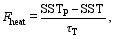
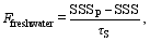
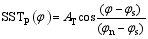
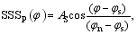
where SST and SSS indicate sea surface temperature and sea surface salinity, respectively; Fheat and Ffreshwater are the surface heat and freshwater fluxes, respectively; and τT and τS are the restoring time scales of temperature and salinity, respectively. Furthermore, SSTP and SSSP are the prescribed restoring SST and SSS with the following forms:
| Table 1 Configurations used in the model. |
where AT and AS are the amplitude of SSTP and SSSP. In addition, φ indicates latitude, with φs= 10°N, φn= 74°N beings the latitudes of the southern and northern boundaries, respectively. Under these restoring conditions, a steady state was reached from a motionless initial state in about 10000 years, using the THCM. The surface heat and freshwater fluxes were diagnosed from this steady state, which were subsequently prescribed as time-independent surface fluxes used to force the model. A further 1000-year simulation showed that the steady state did not change under prescribed conditions for temperature and salinity, thereby remaining (linearly) stable. The prescribed flux conditions for temperature and salinity were used to investigate the decadal THC variability.
The steady state is shown in Fig. 1. The maximum of the meridional overturning stream function (Fig. 1a) was located at (60°N, -1500 m) and was of about 16 Sv (1 Sv = 106m3 s-1). An upwelling (downwelling) was observed near the western (eastern) boundary (Fig. 1b) and a weak density stratification in high latitudes (Fig. 1c) that reflected strong convection. SST (Fig. 1d) ranged from 28°C in the low latitudes to 2°C in the high latitudes, while SSS (Fig. 1e) ranged from 35.4 psu in the low latitudes to 34.6 psu in the high latitudes. Velocities averaged over the upper layers (above -1500 m; Fig. 1f) showed that downwelling mainly occurred near the northeastern boundary and upwelling occurred in the rest of the basin, intensifying near the northwestern boundary. These results were consistent with the background states determined previously using different idealized models ( Sévellec et al., 2009; Zanna et al., 2011; Zu et al., 2013). The steady state, as plotted in Fig. 1, was used as the basic state to compute the CNOP and study decadal variability of the THC.
The CNOP method was used to determine the optimal nonlinear excitation of the decadal THC variability. This method can be used to search the largest-growing initial perturbations in a nonlinear model over a fixed time ( Mu et al., 2003). It has been used to explore the predictability of ENSO events ( Duan and Mu, 2006) and the Kuroshio Large Meander ( Wang et al., 2012), to study the use of adaptive observations for tropical cyclones ( Qin and Mu, 2012), to determine the sensitivity and decadal variability of the THC ( Mu et al., 2004; Sun et al., 2005; Zu et al., 2013), and to assess the sensitivity of ecological systems ( Sun and Mu, 2011), etc.
For a detailed description of the CNOP method, we referred to Mu et al. (2003, 2004). For the computation of CNOP within the THCM, we measured the THC strength using the following objective function:
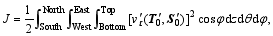
where ν'τ is the meridional velocity anomaly at the time τ induced by the initial temperature or salinity perturbations (T'0, S'0). In Eq. (5), South, North, West, East, Top, and Bottom indicate the boundaries of the ocean domain, and φ, θ? and z are latitude, longitude, and depth, respectively. The objective function J can be used to measure the integral meridional velocity anomalies, which in turn can yield the THC variations.
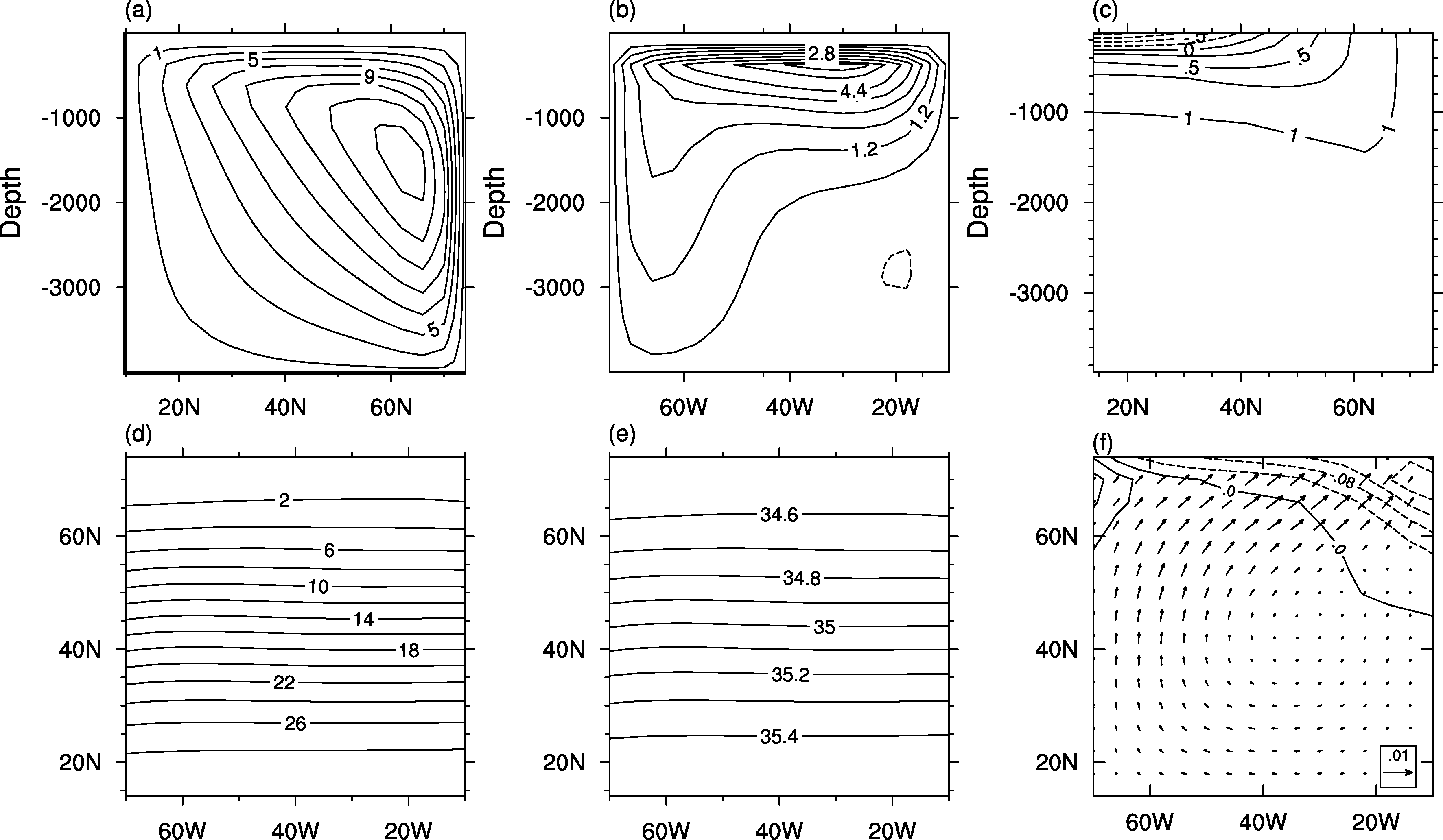 | Figure 1 Steady state: (a) meridional overturning stream function ψ (defined by ; units: Sv), (b) zonal overturning stream function χ (defined by ; units: Sv), (b) zonal overturning stream function χ (defined by ; units: Sv), (c) zonal mean density (units: kg m-3), (d) sea surface temperature (units: °C), (e) sea surface salinity (units: psu), and (f) velocities averaged over upper layers (from sea surface to -1500 m; units: m s-1), with horizontal velocities denoted by arrows and vertical velocities by contours. In these figures, solid and dashed lines denote positive and negative values, respectively. ; units: Sv), (c) zonal mean density (units: kg m-3), (d) sea surface temperature (units: °C), (e) sea surface salinity (units: psu), and (f) velocities averaged over upper layers (from sea surface to -1500 m; units: m s-1), with horizontal velocities denoted by arrows and vertical velocities by contours. In these figures, solid and dashed lines denote positive and negative values, respectively. |
In this study, the initial perturbations of temperature and salinity were regarded as the variations of temperature and salinity, and were allowed anywhere in the 3D ocean basin. The temperature and salinity perturbations were optimized separately, satisfying the constraints 

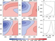
The optimal initial salinity perturbations of CNOP type are shown in Fig. 2. The perturbations presented a 3D pattern; however, in the figure perturbation patterns on only four layers (-125, -1375, -2375, and -3875 m; Figs. 2a, 2b, 2d, and 2e) are shown. The perturbations consisted mainly of negative salinity anomalies located in the northwestern part of the basin. To determine the integral characteristics of these perturbations, we defined an index

to measure the vertical profile of the perturbations and another index

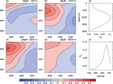
to measure the meridional structure of the perturbation. Here P′ are either temperature or salinity perturbations, and the subscripts xy, xz, and xyz indicate that the sums were taken over zonal and meridional dimensions, zonal and vertical dimensions, and all dimensions, respectively. The perturbations were mainly located at the mid-depth ranging from -1500 to -3000 m (Fig. 2c), with the largest amplitude being near 60°N (Fig. 2d). These perturbations can be regarded as optimal precursors for the decadal THC variability, implying that if the salinity anomalies resembling this structure are imposed in the ocean, for example by overflows, a strong modification (weakening) of the THC will likely occur after a decade. The optimal initial temperature perturbations of CNOP type are shown in Fig. 3. These perturbations were also shown to have their largest amplitudes in the northwestern part of the basin (Figs. 3a, 3b, 3d, and 3e), at about 60°N (Fig. 3f) and near the mid-depth (from -1500 to -2500 m, Fig. 3c). This perturbation pattern can be regarded as the optimal precursor of temperature variations for the THC variability on a decadal time scale.
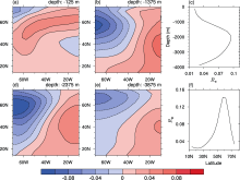
In the model, we used the same type of boundary conditions (prescribed flux conditions) and the same mixing coefficients in the prognostic equations of both temperature and salinity. Spatial patterns of the temperature and salinity perturbations evolved identically, as there was basically only one tracer i.e., density affecting the flow. Hence the two kinds of perturbations showed similar spatial structures. The two types of perturbations exerted a cooperative effect on the density anomalies (Fig. 4). As a result, the density perturbations also showed a similar spatial structure to that of temperature and salinity fields; the largest amplitude of the perturbations was shown in the northwestern part of the basin (Figs. 4a, 4b, 4d, and 4e), at about 60°N (Fig. 4f) and near the mid-depth (from -1500 to -3000 m, Fig. 4c). This indicates that the density anomalies in this region will influence the future changes in the THC significantly, irrespective of whether they are caused by temperature or salinity anomalies. It should be noted that the initial temperature and salinity perturbations, shown in Figs. 2 and 3, were optimized separately. We also optimized these initial perturbations simultaneously, and the results were basically the same as shown in Figs. 2-4, since we used a linear equation of state.
The similar patterns of optimal initial temperature and salinity perturbations indicate that the northwestern basin is a very sensitive area, which is in agreement with the results of Zanna et al. (2011). Hence, the variations of temperature and salinity in this region will likely influence the THC strength on a decadal time scale significantly. Moreover, the largest amplitude of the perturbations were found to be located at mid-depths, instead of being near the surface, indicating the perturbations at depth in the northwestern part of the basin to be much more efficient at exciting the THC modifications on a decadal time scale than those at other locations. Actually, the sensitive area corresponded to the south of Greenland and Labrador Sea, which indeed present strong variability of temperature and salinity in the deep ocean, according to SODA. Therefore, this localized temperature and salin ity variability may be responsible for the decadal THC modifications due to inherent physics. From a prediction point of view, increasing observational effort in these regions to monitor the variations of temperature and salinity at depth may be an efficient way to improve the forecast skill of THC variability on a decadal time scale.
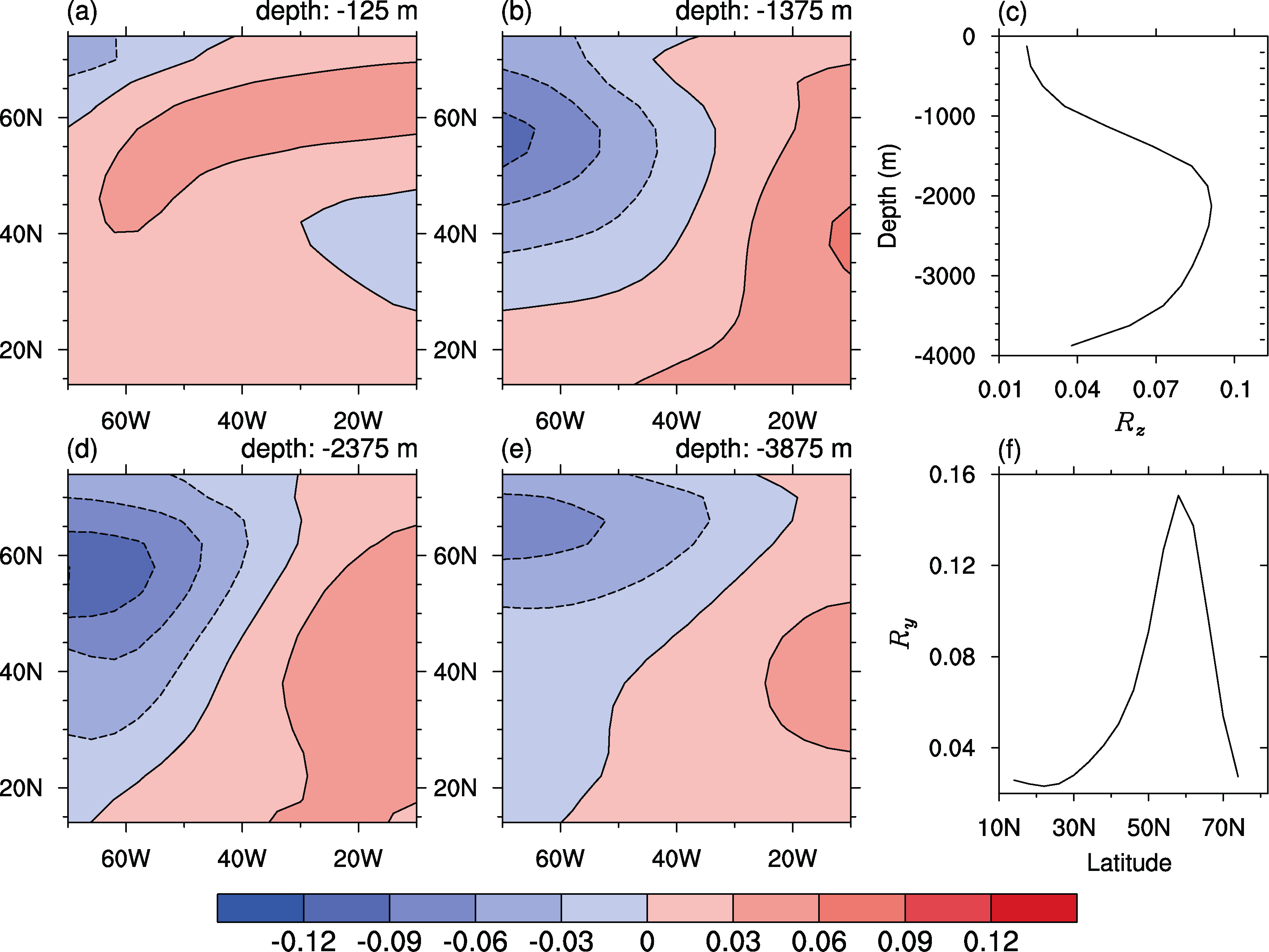 | Figure 2 Optimal initial salinity perturbations on the layers of (a) -125 m, (b) -1375 m, (d) -2375 m, and (e) -3875 m (units: psu), and the indices of (c) Rz and (f) Ry defined in Eqs. (6) and (7), respectively. |
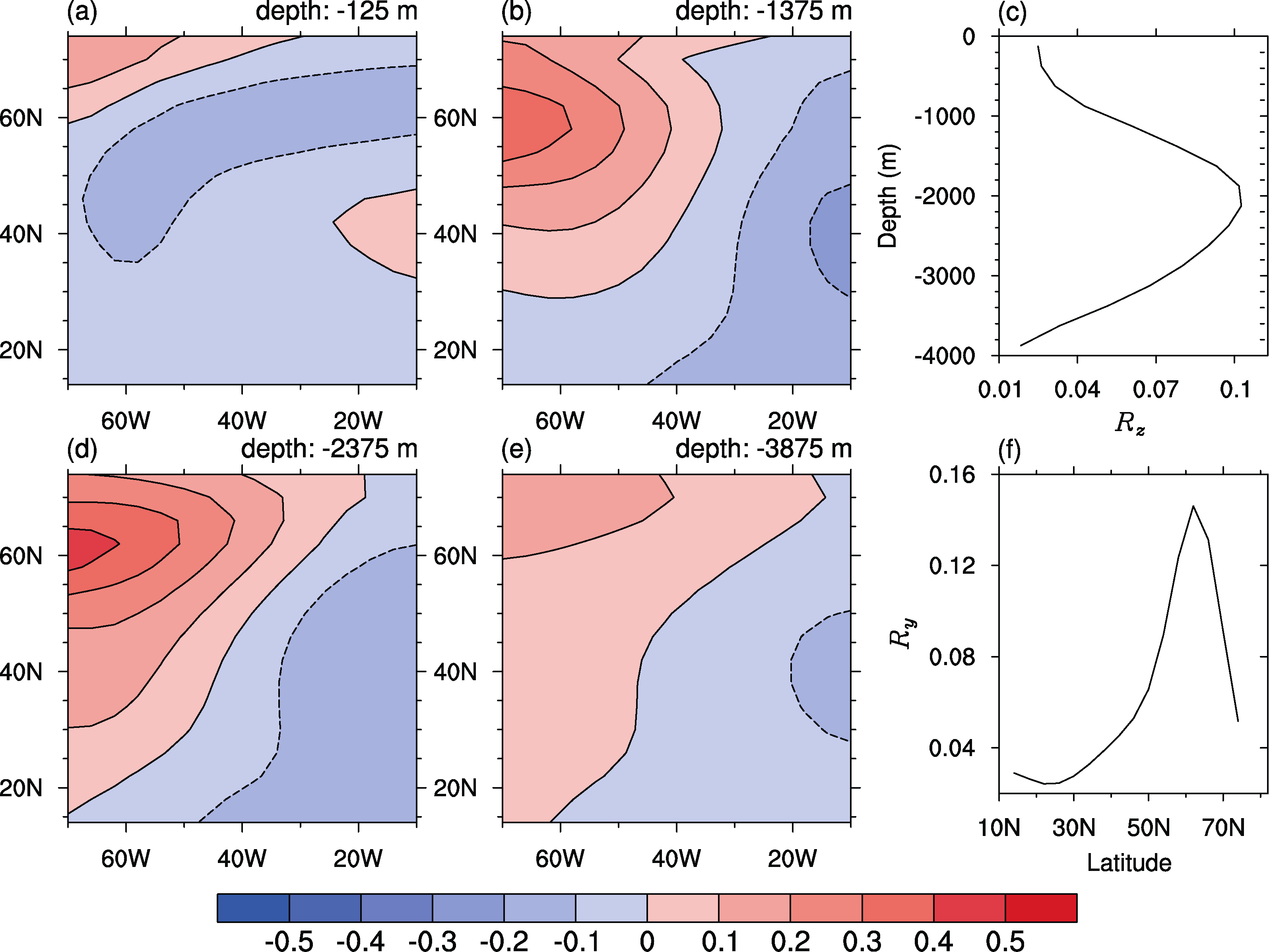 | Figure 3 Optimal initial temperature perturbations on the layers of (a) -125 m, (b) -1375 m, (d) -2375 m, and (e) -3875 m (units: °C), and the indices of (c) Rz and (f) Ry defined in Eqs. (6) and (7), respectively. |
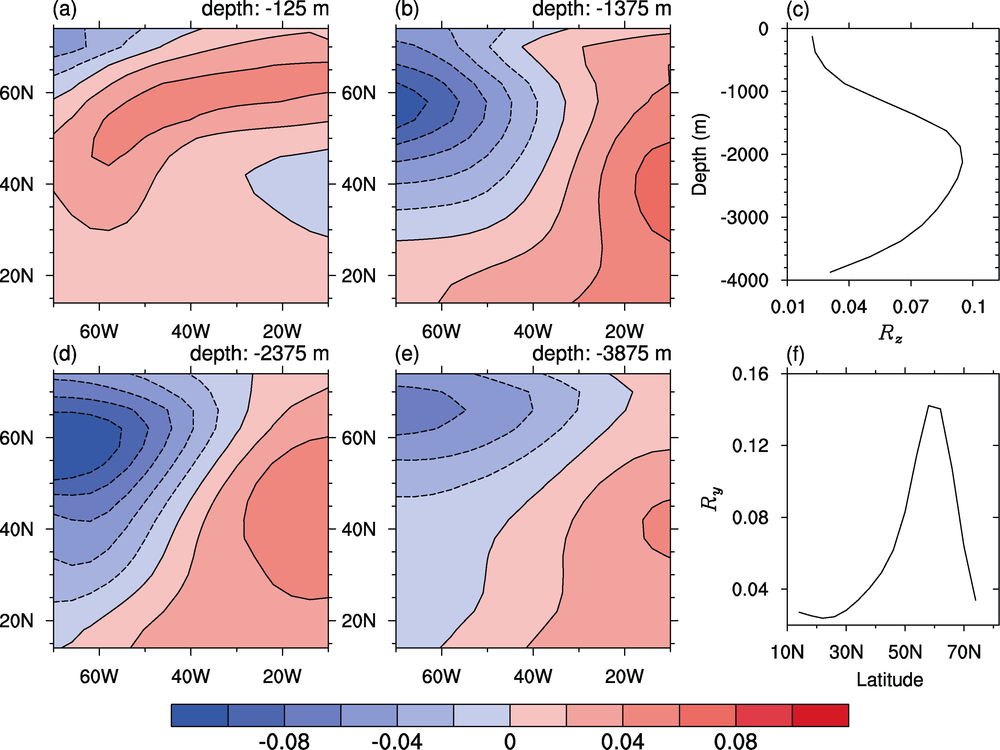 | Figure 4 Initial density perturbations (caused by optimal initial perturbations of temperature and salinity) on the layers of (a) -125 m, (b) -1375 m, (d) -2375 m, and (e) -3875 m (units: kg m-3), and the indices of (c) Rz and (f) Ry defined in Eqs. (6) and (7), respectively. |
We investigated the decadal THC variations induced by the optimal initial perturbations of temperature and salinity. This variability was calculated by superimposing the perturbations on the basic state at the initial time and then integrating the model forward in time for decades (indicated by the nonlinear evolution of the perturbations in the following). To assess the importance of nonlinear processes, we also calculated the decadal THC variations using a forward integration with the tangent linear model initialized by the optimal perturbations (indicated by the linear evolution in the following).
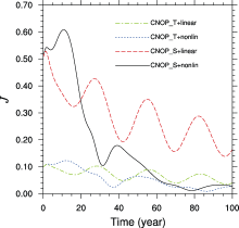
To show the THC variability, we plotted the objective function (Eq. (5)) versus time. The decadal THC variations induced by the optimal initial perturbations are shown in Fig. 5. The nonlinear evolution of the optimal salinity perturbations (represented by the black solid curve in Fig. 5) indicates that the objective function increased abruptly and then decreased quickly with weak and irregular oscillations. The nonlinear evolution of optimal temperature perturbations (represented by the dotted blue curve in Fig. 5) was found to show similar characteristics, but the amplitude of the decadal variability was much smaller. Since the absolute maxima of the optimal perturbations were considered as the realistic amplitude of the variations of temperature and salinity, the decadal variations of the THC simulated in this study represented the upper bound caused by all kinds of perturbations of temperature and salinity, of course ignoring the model errors. Hence, in reality, salinity variations play a more important role in exciting decadal THC variations than temperature variations.
Compared with the nonlinear evolutions of these perturbations, the linear evolutions (Fig. 5) showed significantly different characteristics. In the tangent linear model, the objective functions were shown to decrease slowly and oscillate regularly over a period of roughly 30 years. It implies that a damped oscillatory eigenmode determined by thermal wind relation was likely excited and dominated the linear evolution of the perturbations ( Te Raa and Dijkstra, 2002). The difference in values of the objective function between the linear and nonlinear evolution cases was significant, mainly due to the (nonlinear) convection, indicting that taking nonlinear processes into account will influence the development of perturbations significantly. Hence, nonlinear processes are important for determining the THC variability.
 | Figure 5 Decadal THC variations measured by objective function J( t) in the nonlinear model initialized by optimal temperature (CNOP_T + nonlinear) and salinity (CNOP_S + nonlinear) perturbations and in the tangent linear model initialized by optimal temperature (CNOP_T + linear) and salinity (CNOP_S + linear) perturbations. |
In this study, we determined the 3D structure of the optimal initial perturbations of temperature and salinity within a 3D idealized ocean circulation model, using the CNOP method. Nonlinear characteristics of the decadal THC variability excited by these perturbations were investigated. Unlike in the previous works, in our study the perturbations were allowed anywhere in the 3D ocean basin, rather than being confined to the sea surface.
The largest amplitudes of the optimal perturbations of both temperature and salinity were reported to be located at depths ranging from -1500 to -3000 m in the northwestern part of the basin. Such perturbations can, for example, be caused by overflows or deep convection and are likely more efficient to excite the decadal variability of the THC than those on the sea surface and hence can be regarded as the optimal precursor or early warning indicator of future changes of the THC. Therefore, increasing observational effort in the northwestern part of the Atlantic to monitor the variations of temperature and salinity at depth would be an efficient way to improve the forecast skill of the THC variability on a decadal time scale.
The decadal THC variations induced by the optimal salinity perturbation were found to be much stronger than those caused by optimal temperature perturbations. Hence, the salinity perturbations might be expected to play a relatively important role in exciting the decadal THC variations, as the absolute maxima of the optimal perturbations were considered as realistic amplitudes of the variations of temperature and salinity. Moreover, the linear and nonlinear evolutions of the optimal initial salinity perturbations showed remarkable differences, suggesting important contributions from nonlinear processes to decadal THC variability. A more detailed explanation of the perturbation growth is considered outside the scope of this paper.
Most researchers have focused on the effects of SST and SSS on the excitation of THC variability. These studies are reasonable, because the variations of SST and SSS show relatively large amplitude due to the influence of atmospheric forcing. Although strong variations of SST and SSS can cause decadal THC variability, they are not likely the most efficient factors. In contrast, the relatively weak variations of temperature and salinity at mid-depth may have a stronger potential to excite decadal THC variability. In our study, it was difficult to quantify the differences between the effects of strong surface variations and weak mid-depth variations. However, we found the mid-depth variations to have a stronger influence than the surface variations with the same amplitude. Hence, for the forecast of decadal THC variations, the relatively weak variations of temperature and salinity in the initial conditions at mid-depth should not be ignored, since they likely play an important role. In addition, the perturbations were found not to spread uniformly at mid-depth, but to be localized in the northwestern part of the basin. It suggests that observations in this localized region, rather than those uniformly distributed over the basin, can likely provide initial conditions to improve forecasts of decadal THC variability efficiently.
| 1 |
|
| 2 |
|
| 3 |
|
| 4 |
|
| 5 |
|
| 6 |
|
| 7 |
|
| 8 |
|
| 9 |
|
| 10 |
|
| 11 |
|
| 12 |
|
| 13 |
|
| 14 |
|
| 15 |
|
| 16 |
|
| 17 |
|
| 18 |
|
| 19 |
|
| 20 |
|
| 21 |
|
| 22 |
|