

Projections of Global Mean Surface Temperature Under Future Emissions Scenarios Using a New Predictive Technique
[WANG Ge-Li , YANG Pei-Cai]
, YANG Pei-Cai]
|
|


Using numerical model simulations, global surface temperature is projected to increase by 1°C to 4°C during the 21st century, primarily as a result of increasing concentrations of greenhouse gases. In the present study, a predictive technique incorporating driving forces into an observation time series was used to project the global mean surface temperature under four representative scenarios of future emissions over the 21st century.
Predictions of temperature rise during the 21st century are uncertain. This is because the sensitivity of the climate system to changing atmospheric greenhouse gas concentrations, as well as the rate of ocean heat uptake, are poorly quantified; and also because future influences on the climate of anthropogenic, as well as natural origin, are difficult to predict ( Stott and Kettleborough, 2002).
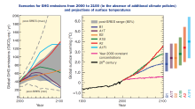
The Intergovernmental Panel on Climate Change (IPCC), in their Special Report on Emissions Scenarios (SRES), has developed a wide range of future emissions scenarios. Multi-model averages and assessed ranges for surface warming are presented in Fig. 1. In the IPCC (2007) report, approximate CO2 equivalent concentrations corresponding to the computed radiative forcing due to anthropogenic greenhouse gases and aerosols in 2100 for the SRES B1, A1T, B2, A1B, A2, and A1FI illustrative marker scenarios are approximately 600, 700, 800, 850, 1250, and 1550 ppm, respectively. Scenarios B1, A1B, A2, and 20C have been the focus of model intercomparison studies and many of these results are assessed in the report. Models predict that by 2100 the global mean surface temperature change will be 1.0°C to 4°C.
Climate models are mathematically-based models that attempt to calculate the climate, its variability, and its systematic changes on a first-principles basis. On timescales of 10-50 years (and longer), decadal climate forecasts are difficult to make with general circulation climate models due to their many uncertainties, such as model resolution and land-use or vegetation feedback ( Gao et al., 2003, 2006; Jiang et al., 2011).
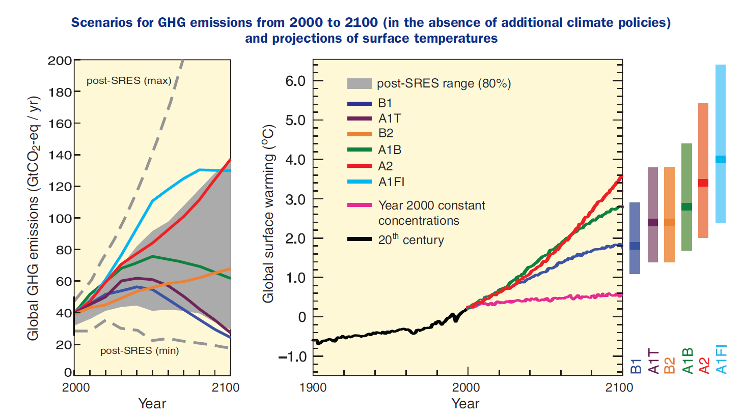 | Figure 1 Scenarios for Green House Gases (GHG) emissions from 2000 to 2100 (in the absence of additional climate policies) and projections of surface temperatures. Left panel: Global GHG emissions (in GtCO2-eq) in the absence of climate policies: six illustrative Special Report on Emissions Scenarios (SRES) marker scenarios (colored lines) and the 80th percentile range of recent scenarios published since SRES (post-SRES) (gray shaded area). Dashed lines show the full range of post-SRES scenarios. The emissions include CO2, CH4, N2O, and F-gases. Right panel: Solid lines are multi-model global averages of surface warming for scenarios A2, A1B, and B1, shown as continuations of the 20th century simulations. These projections also take into account emissions of short-lived GHGs and aerosols. The pink line is not a scenario, but represents Atmosphere-Ocean General Circulation Model (AOGCM) simulations, where atmospheric concentrations are held constant at year-2000 values (from IPCC (2007)). |
A compatible approach to numerical model simulations for assessing recent climate change and forecasting future change is the direct analysis of surface temperature observations. We incorporated external forces to establish a nonlinear time series prediction to develop global surface temperature projections for the 21st century under the same scenarios as SRES provided by IPCC (2007).
The following section gives a brief introduction to the algorithm for establishing the prediction model. Results from prediction experiments on global temperature variation incorporating greenhouse gas emissions defined by SRES and solar irradiation are presented next. We finish by providing a brief discussion of the results.
The dynamics of the reconstructed trajectory is equivalent to that of the original system that generated the time series, and it is now common practice to use this time series and its successive time shifts (delays) as coordinates of a vector time series, based on this trajectory, enabling the establishment of a model to predict the future state of the system.
For convenience, we assume a non-stationary process composed of three series, 


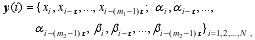
or simply as
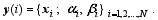
Here, m1and m2 are the given embedding dimensions for 


where fp is some desired mapping, assumed to be a quadratic polynomial in this study; 
present study. The next task is to find the cost function, 
The above approach is successful in improving prediction when forcings are included in "ideal" stationary systems, such as the Lorenz system, a logistic model, or global temperature over seasonal timescales, including the North Atlantic Oscillation (NAO), the Pacific Decadal Oscillation (PDO), the El Niño/Southern Oscillation (ENSO), and the North Pacific Index (NPI), variability, which suggests that these major climate modes or forcings play a significant role in influencing the global temperature over decadal time scales ( Wang and Yang, 2010; Wang et al., 2012). In the present study, the approach was extended to project the global temperature throughout the rest of the 21st century.
Using the above approach, and recent data comprising 160 years of global annual mean surface temperature variations, a projection of global temperature variations for the 21st century was produced. The aim of the 20-year (1991-2010) annual temperature variation prediction experiment was to illustrate and test the new approach.
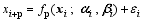
Data were divided into two parts: the preceding 140 points were applied to construct the predictive model, and the following 20 points were used to test the accuracy of the prediction. The global mean surface air temperature variation was predicted for 1991-2010. The parameters used for building the model were assigned the following values: the time lag, τ, was 1; the embedding dimensions of Ti and m1 were taken from 3 to 7; and the embedding dimensions of all four of the driving forces of m2 were set to be either 0 (for external forcings not considered) or in the range from 3 to 5 (for external forcings considered). The results were averaged over the embedding dimensions, and the prediction results of the global mean surface air temperature variation with or without driving forces and observation values are shown in Fig. 2. Figure 2a gives the comparison between observation and prediction for this period; Fig. 2b gives the error between the observation and prediction depending on the prediction step; and Fig. 2c shows the dependence of the root- mean-square error (RMSE) on the prediction steps during the period 1991-2010 with or without considering external forcings. It can be seen that the RMSE values that incorporate forcings were much lower than those without forcings, and also the growth in the error rate for prediction steps with forcings was lower than that without forcings. This illustrates again that the introduction of driving forces to prediction models can yield an obvious improvement in their accuracy, and also gives us the confidence to project the global temperature variation under the different scenarios.
 | Figure 2 (a) Predictive comparison between observation and prediction during 1991 to 2010; (b) Error observation and prediction; (c) RMSE dependent on prediction steps with or without forcings input. |
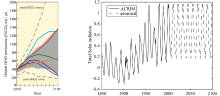
Experiments were performed to project the global mean temperature variation over the 21st century under four representative scenarios for future greenhouse gas emissions (B1, A1B, A2, 20C) provided by IPCC (2007) and solar radiation data provided by the Active Cavity Radiometer Irradiance Monitor Satellite (ACRIM, which monitors total solar irradiance). It was assumed that solar activity will obey an 11-yr period over the next 100 years. Figure 3 shows the external forcings taken into account in the study; the same global greenhouse gas emissions for different scenarios were used in the experiments (see left graph). However, for the solar activity, the 11-yr period variability was assumed from 2010 to 2100, relying on the last 11 values from ACRIM (see right panel of Fig. 3).
 | Figure 3 External forcings controlled in the experiments. The left panel shows the same scenarios for global greenhouse gas emissions as IPCC (2007). The right panel shows the solar activity considered in this study; the solid line represents observations by Active Cavity Radiometer Irradiance Monitor Satellite (ACRIM); the dashed line is the assumption over the remainder of the century. |
The parameters used for building the model were all set to the same values as the above experiments. The projection results under different scenarios (B1, A1B, A2, 20C) are shown in Fig. 4. It can be seen that the results have the same trend as the results in IPCC (2007), but the magnitude of the warming over the 21st century is not as high as the results in IPCC (2007). Our results suggest that the global mean surface temperature variation may increase by 0°C to 1.5°C during the 21st century under the four different scenarios.
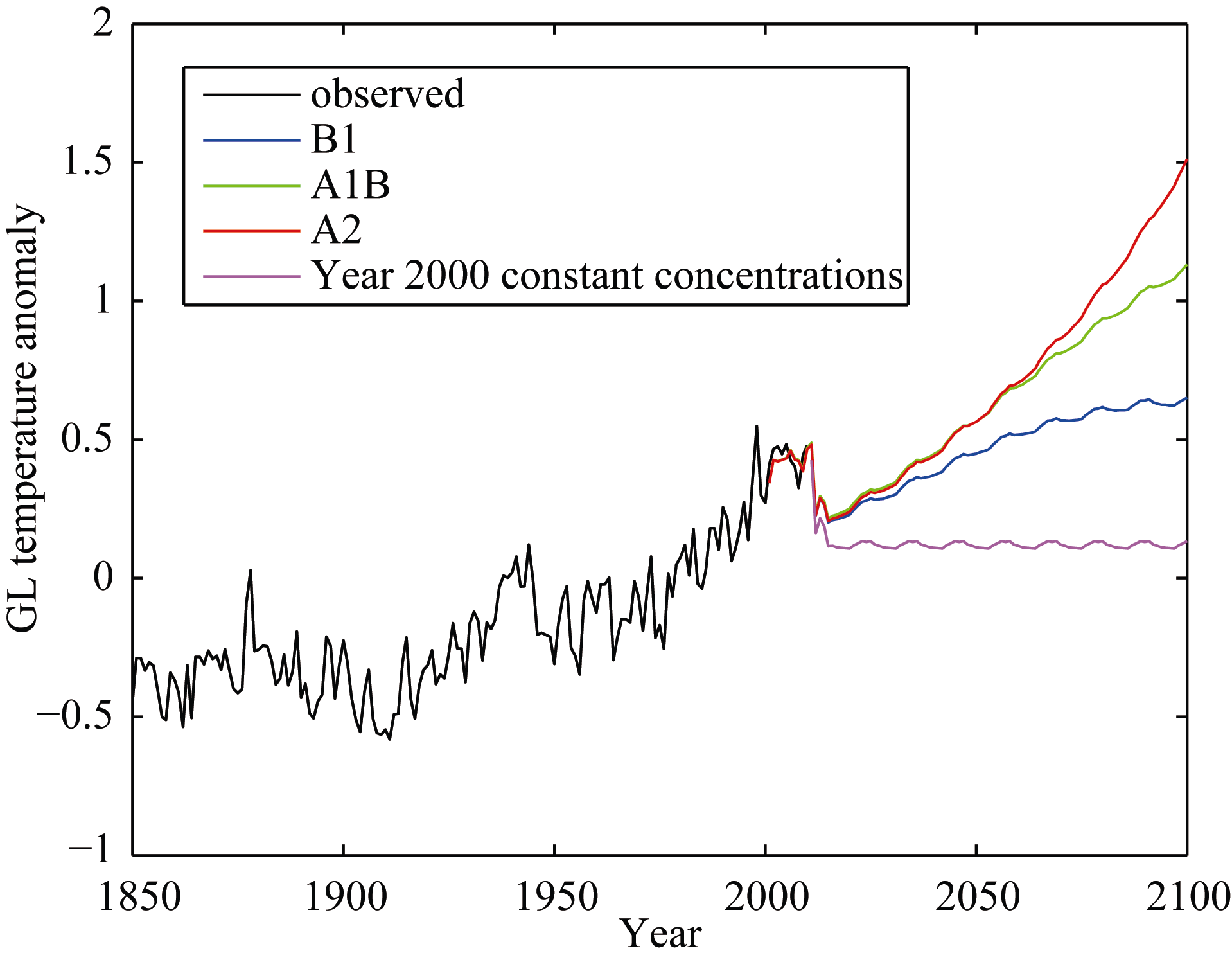 | Figure 4 Projection of global mean temperature variation over the 21st century. |
During the 20th century, the global surface temperature increased by 0.7°C, and it is projected to increase by a further 1°C to 4°C during the 21st century, primarily as a result of increasing concentrations of greenhouse gases ( IPCC, 2007). The IPCC points out that continued greenhouse gas emissions at or above current rates will cause further warming and induce many changes in the global climate system during the 21st century, which are very likely be larger than those observed during the 20th century. In the present reported work, we attempted to develop a compatible approach to numerical model simulations to project global mean temperatures under four representative scenarios of future emissions over the 21st century using global temperature time series. The results suggest that global mean temperatures may rise by 0°C to 1.5°C under the four representative scenarios of future emissions. It is also noted that this approach is needed for a further study on new emissions scenarios of the Representative Concentration Pathways.
Nonlinear prediction is generally successful in identifying chaos and nonlinearity in data because it uses all available points, unlike other methods that exploit only a subset of available points in the attractor ( Sugihara and May, 1990 , Feng et al., 2012). Predictions of global mean temperature over a long timescale are very uncertain, both because the climate possesses significant internal variability, and also because the sensitivity of the climate system to natural and anthropogenic effects is difficult to predict.
Such an approach as that presented here may provide a compatible and direct window to study external forcings of the climate. Work in this area is in progress and will be reported in future publications.
| 1 |
|
| 2 |
|
| 3 |
|
| 4 |
|
| 5 |
|
| 6 |
|
| 7 |
|
| 8 |
|
| 9 |
|
| 10 |
|
| 11 |
|
| 12 |
|