Quantile Trends in Temperature Extremes in China
Cite this Article
FAN Li-Jun. Quantile Trends in Temperature Extremes in China. Atmospheric and Oceanic Science Letters, 2014, 7(4): 304-308 
Permissions
Copyright?2014, Editorial office of Atmospheric and Oceanic Science Letters
This is an Open Access article under the terms of CCAL.
Quantile Trends in Temperature Extremes in China
Abstract
A number of recent studies have examined tre-nds in extreme temperature indices using a linear regression model based on ordinary least-squares. In this study, quantile regression was, for the first time, applied to examine the trends not only in the mean but also in all parts of the distribution of several extreme temperature indices in China for the period 1960-2008. For China as a whole, the slopes in almost all the quantiles of the distribution showed a notable increase in the numbers of warm days and warm nights, and a significant decrease in the number of cool nights. These changes became much fas-ter as the quantile increased. However, although the num-ber of cool days exhibited a significant decrease in the mean trend estimated by classical linear regression, there was no obvious trend in the upper and lower quantiles. This finding suggests that examining the trends in different parts of the distribution of the time-series is of great importance. The spatial distribution of the trend in the 90th quantile indicated that there was a pronounced increase in the numbers of warm days and warm nights, and a decrease in the number of cool nights for most of China, but especially in the northern and western parts of China, while there was no significant change for the number of cool days at almost all the stations.
Keyword:
extreme temperature indices; quantile trend; quantile regression; China
1 Introduction
In the last few decades, extreme weather and climate events have attracted wide attention because of their huge impact on human life, the environment, the economy, and society (Intergovernmental Panel on Climate Change (IPCC), 2012). Also, Katz and Browns (1992) found that extreme events are more important than averages in changing climate.
A number of extreme climate indices have been developed to examine the observed change in extremes ( Jones et al., 1999; Klein Tank and Können, 2003). During the past few years, numerous studies of trends in extreme temperature indices have been carried out in various regions of the world ( Klein Tank and Können, 2003; Vincent and Mekis, 2006).
In China, a large number of studies of extreme temper-ature indices have been carried out ( Zhai and Ren, 1997; Ren and Zhai, 1998; Yan and Yang, 2000; Wang et al., 2003; Tang et al., 2005; Ren et al., 2005, 2010a, b; Qian et al., 2007, 2012; Zhang et al., 2008; Chen et al., 2009; Ding et al., 2010). These studies concluded that there is a significant increase in the mean maximum temperature in the north of China but no obvious trend in the south; in terms of the mean minimum temperature, there is a consistently significant increase in China and the most remarkable increase is located in the north ( Tang et al., 2005; Zhou and Ren, 2010; Ren et al., 2010a). Besides, increasing trends are detected in the frequencies of warm days and warm nights, and decreasing trends are found in the frequencies of cool days and cool nights ( Zhai and Pan, 2003; Ren et al., 2010a; Zhou and Ren, 2010).
However, in most of the studies above, the trends in extreme temperature indices were often assessed using a classical linear trend model based on ordinary least squ-ares (LSM). Despite the popularity of analyzing linear trends, LSMs still have some limitations. They only provide information about the slope of the mean. When attention is paid to the upper, lower, and all quantiles of the conditional distribution of these extreme indices rather than the mean, the desired information cannot be provided by a LSM ( Tareghian and Rasmussen, 2012).
Fortunately, quantile regression (QR) has been developed as an extension to the LSM approach for estimating the trends not only in the mean but in all parts of the conditional distribution of a variable ( Koenker and Basset, 1978). Compared with LSM, QR can provide a more complete picture of relationships between variables ( Lee et al., 2013). QR analysis has been widely used in a number of social studies (e.g., McGuinness and Bennett, 2007). However, this technique has only recently been used in climate change research ( Barbossa, 2008; Tareghian and Rasmussen, 2012; Lee et al., 2013).
This paper introduces the QR method for the first time to investigate trends in all parts of the conditional contributions of extreme temperature indices in China, rather than the trend in the mean. In addition, the trends in the lower, median, and upper quantiles were also compared with that in the mean of each index estimated by LSM in order to explain the advantage of the QR method over LSM.
2 Data and extreme temperature indices
The homogenized daily maximum ( Tmax) and minimum ( Tmin) temperature data at 549 stations in China during the period 1960-2008 were employed in this study ( Li and Yan, 2009).
A set of four indices of temperature extremes was selected for this study (Table 1). These four indices were based on thresholds defined as percentiles; therefore, they are effective at any station and in any season. They were calculated on an annual basis at each individual station. The 10th and 90th percentiles were calculated for every day of the calendar year during the 1961-1990 reference periods ( Zhai and Pan, 2003). Note that these four indices did not necessarily represent extreme warm days and nights in the summer or extreme cool days and nights in the winter.
Because of the nonuniform spatial distribution of the stations, eastern China with a higher density of stations is usually overrepresented in the China average. Therefore, a simple approach was adopted to compute the China mean time series for the four extreme indices. The whole domain was divided into 2° × 2° grid boxes. The average value was calculated from all stations within a grid box, and then the China mean value was computed from all the box values ( Vincent and Mekis, 2006). We did not consider 2° × 2° grid boxes that did not contain a station.
3 Quantile regression
QR can be considered as an extension of LSM. Within the LSM framework, the response variable ( Y) is linearly correlated with time ( t): Y = αt + β, with α representing the linear slope and β the intercept. The parameters α and β are assessed by the ordinary least-squares estimate of the mean of the response variable Y conditional on t ( E( Y| t)), and obtained by minimizing the sum of squared residuals.
QR can be easily understood by replacing E( Y| t) by the quantile of the response variable Q( τ| t). For each quantile, τ, the linear quantile regression model can be described as Y = f'( α τ, β τ, t), with α τdenoting the quantile slopeand β τthe intercept for each τ. Rather than LSM, these two parameters can be estimated from the conditional quantile function by minimizing the sum of asymmetrically weighted absolute residuals:
| (1) |
where
A detailed description of the QR method can be found in previous papers ( Barbosa, 2008; Tareghian and Rasmussen, 2012; Lee et al., 2013).
The QR method was employed to estimate the trends in different quantiles of the four indices for the China mean and 549 stations, respectively. LSM was employed to estimate the mean trend of the four China mean indices. Their statistical significances were tested at the 95% confidence level using the t-test. The trends in the upper, median, and lower quantiles were compared with the mean trend. The slopes in the 90th quantile were gridded with spline interpolation and mapped in order to explore their spatial distribution characteristics. Note that the interpolation process did not consider the topographic correction (Xu et al., 2009; Wu and Gao, 2013).
| Table 1 The four extreme temperature indices (units: number of days) used in this study. |
4 Results
4.1 Quantile trends of China mean indices
Figure 1 displays the trends in the 10th, 50th, and 90th quantiles estimated by QR and the mean estimated by LSM for the four extreme indices. The trends in the mean and 50th quantile can be understood as the measurement of the central tendency for the four extreme indices, whereas those in the 10th and 90th quantiles reflect the variability in their lower and upper extreme parts. For the number of warm days, although an increasing trend similar to the mean trend was detected in the 10th, 50th, and 90th quantiles, their slopes were significantly different. The slope in the 90th quantile (5.82 days per decade) was much greater than that in the mean (4.70 days per decade), whereas the slope in the 10th quantile (2.39 days per decade) was smaller than the mean slope (Fig. 1a). For the number of cool days, a consistent decreasing trend was found in the median quantile (-0.90 days per decade) and the mean (-0.58 days per decade); however, the lines of the trends in the 10th (0.19 days per decade) and 90th (0.07 days per decade) quantiles were almost parallel, suggesting that although the mean variability decreased, the variability in the extreme quantiles did not change dramatically (Fig. 1b). For the number of warm nights, there was a significant increase in the upper quantile (8.83 days per decade), which was almost the same as those in the mean (8.46 days per decade) and median quantile (8.15 days per decade), whereas the slope in the lower quantile (4.63 days per decade) was much lower than the slope in the mean and upper quantiles (Fig. 1c). As for the number of cool nights, there was a sharply decreasing trend in the three quantiles and the mean, and the trend in the upper quantile (-4.59 days per decade) was more significant than the others (Fig. 1d).
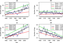
The quantile slopes estimated by QR for quantiles 0.01 to 0.99 (in steps of 0.01) are displayed in Fig. 2. In contrast to the mean slope estimated by LSM (red lines), QR shows a more complete view (black dots) of the change of the distribution for the four China mean indices. For the number of warm days, the confidence envelopes of the slopes of the quantiles greater than 0.2 did not cross the zero line, suggesting that increasing trends are statistically significant for all the quantiles larger than 0.2 (Fig. 2a). Similarly, the number of warm nights showed statistically significant increasing trends in the quantiles greater than 0.1 (Fig. 2c). Meanwhile, the quantile slopes of these two indices increased as the quantile increased. In contrast, the number of cool nights indicated statistically significant negative slopes for all quantiles and the slopes decreased as the quantile increased (Fig. 2d). For the number of cool days, although there was a significant decreasing trend in the quantiles 0.3 to 0.7, the trends in the upper (higher than 0.7) and lower (lower than 0.3) quantiles exhibited no obvious change (Fig. 2b).
To summarize, the trends of the four indices in the median were very near to those in the mean, whereas the upper and lower quantiles showed significantly different trends from those in the mean. More interestingly, the upper extreme parts of the numbers of warm days, warm nights, and cool nights changed more rapidly than the other quantiles and the mean trend, and therefore more attention should be paid to these.
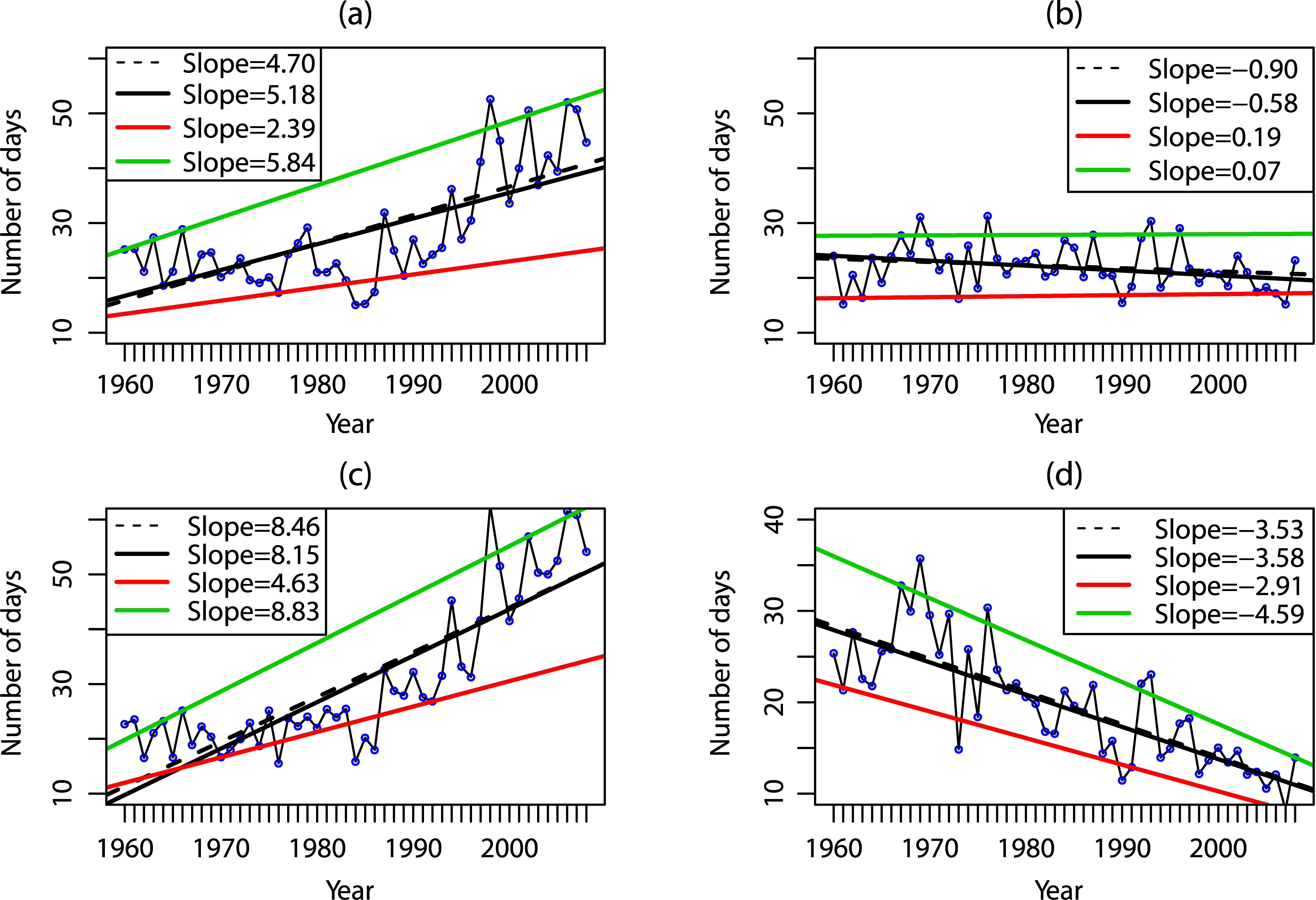 | Figure 1 Trends in the 10th (red lines), 50th (black lines), and 90th (green lines) quantiles estimated by quantile regression (QR) and the mean (black dotted lines) estimated by LSM for the four China mean temperature indices: (a) warm days; (b) cool days; (c) warm nights; and (d) cool nights. The slopes (units: days per decade) are the trends in the three quantiles and the mean. |
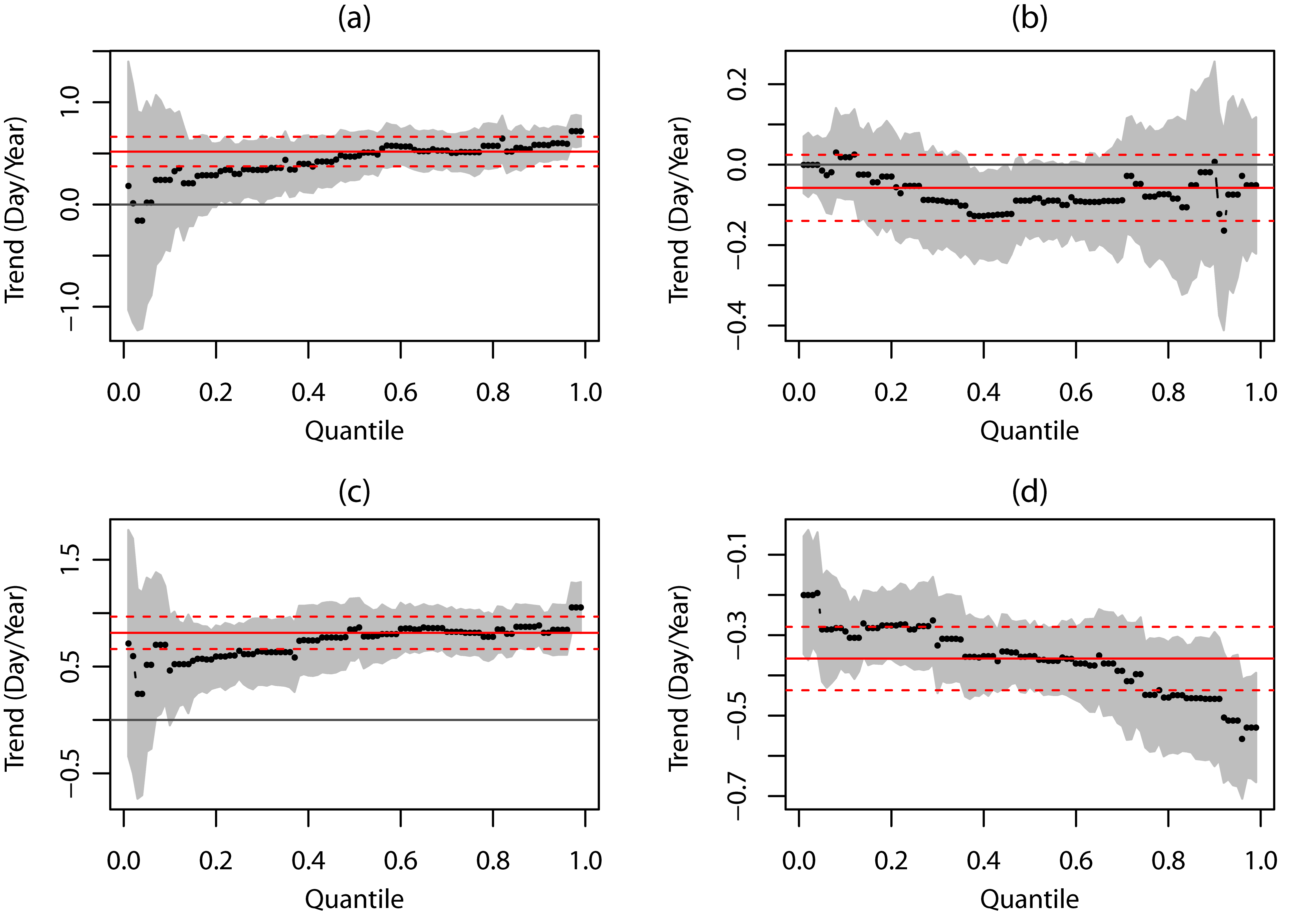 | Figure 2 The quantile regression coefficients (black dots) for the quantiles from 0.01 to 0.99 in increments of 0.01 and their 95% confidence levels (shaded in grey) for the four indices: (a) warm days; (b) cool days; (c) warm nights; and (d) cool nights. The solid red line is the mean trend estimated by LSM and dashed red lines indicate the 95% confidence levels. |
4.2 Spatial distribution of quantile trends
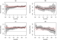
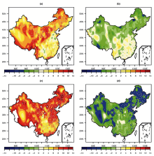
The quantile trends were analyzed by the QR method for the 549 stations and the four indices. Figure 3 shows the spatial distributions of the slopes for only the 90th quantile. For most of the spatial domain, notably in the northern and western parts of China, the number of warm days showed a significant increasing trend greater than 2 days per decade (Fig. 3a). A more pronounced increasing trend was found in the number of warm nights, especially those in the northern and western parts of China, with the trend greater than 8 days per decade (Fig. 3c). In contrast, the number of cool days indicated no significant decreasing trend in the whole of China apart from a very few number of stations. This finding is totally different from the mean trend, which suggested a significant decline at most of the stations (Fig. 3b). For the number of cool nights, there was a remarkable decrease in most parts of China, especially for those in northeastern China with slopes smaller than -6 days per decade (Fig. 3d).
5 Conclusion
The QR method was applied to study the trend of the conditional distribution for the four indices of temperature extremes in China. Compared with classical linear regression, the QR method was able to provide a more complete analysis of the long-term temporal variability of the conditional distribution for each index. As the quantile increased, the more notably increasing trend was observed for the frequencies of warm days and warm nights, and the more remarkably decreasing trend was found for the frequency of cool nights. Meanwhile, the change in the 90th quantile was the most remarkable in the northern and western part of China for these three indices.
In addition, the advantage of the QR method can be well embodied in the analysis of the number of cool days.
 | Figure 3 The 90th quantile slopes (units: days per decade) estimated by the QR method for the four indices: (a) warm days; (b) cool days; (c) warm nights; and (d) cool nights. Grey dots denote the stations where the trend is statistically at the 95% confidence level. |
The slopes in the upper and lower quantiles suggested a totally different change from those of the middle quantiles and the mean. The mean trend estimated by the LSM method showed a significant decreasing trend, which is consistent with the studies of Zhai and Pan (2003) and Zhou and Ren (2010). The result reported in this paper reveals that there are no significant trends in the upper and lower quantiles for the frequency of cool days. The change in the tail of the distribution is always more valuable than the mean slope for climate risk assessment. Therefore, the QR method is a very useful tool for identifying the trends of all parts of the conditional distribution of a time series and should be considered for the study of climatic long-term variability.
Acknowledgements. This work was jointly sponsored by the National Basic Research Program of China (973 Program, Grant No. 2012CB956203), the Knowledge Innovation Project of the Chinese Academy of Sciences (Grant No. KZCX2-EW-202), and the Strategic Priority Research Program of the Chinese Academy of Sciences (Grant No. XDA05090100).
Reference
| 1 |
|
| 2 |
|
| 3 |
|
| 4 |
|
| 5 |
|
| 6 |
|
| 7 |
|
| 8 |
|
| 9 |
|
| 10 |
|
| 11 |
|
| 12 |
|
| 13 |
|
| 14 |
|
| 15 |
|
| 16 |
|
| 17 |
|
| 18 |
|
| 19 |
|
| 20 |
|
| 21 |
|
| 22 |
|
| 23 |
|
| 24 |
|
| 25 |
|
| 26 |
|
| 27 |
|
| 28 |
|