Verifying Fossil-Fuel Carbon Dioxide Emissions Forecasted by an Artificial Neural Network with the GEOS-Chem Model
[WANG Yi-Nan1, 2 , L#cod#x000dc; Da-Ren1, *  , LI Qian
1 , PAN Yu-Bing1, 2 ]
, LI Qian|
|


In this study, the authors developed an ensemble of Elman neural networks to forecast the spatial and temporal distribution of fossil-fuel emissions (ff) in 2009. The authors built and trained 29 Elman neural networks based on the monthly average grid emission data (1979-2008) from different geographical regions. A three-dimen-sional global chemical transport model, Goddard Earth Observing System (GEOS)-Chem, was applied to verify the effectiveness of the networks. The results showed that the networks captured the annual increasing trend and interannual variation of ff well. The difference between the simulations with the original and predicted ff ranged from -1 ppmv to 1 ppmv globally. Meanwhile, the authors evaluated the observed and simulated north-south gradient of the atmospheric CO2 concentrations near the surface. The two simulated gradients appeared to have a similar changing pattern to the observations, with a slightly higher background CO2 concentration, ~ 1 ppmv. The results indicate that the Elman neural network is a useful tool for better understanding the spatial and temporal distribution of the atmospheric CO2 concentration and ff.
Fossil-fuel emissions (ff) caused by anthropogenic activities is the most important contributor to the increasing concentration of carbon dioxide in the Earth's atmosphere. Denman et al. (2007) investigated the north-south gradient of atmospheric CO2 concentration, and found that annual emissions of CO2 from fossil-fuel burning and cement production increased from a mean of 6.4 ± 0.4 Gt C yr-1 (1 Gt C = 1015 g C) in the 1990s to 7.2 ± 0.3 Gt C yr-1 for 2000 to 2005. In recent years, the emissions have increased to 8-9 Gt C yr-1( Le Quere et al., 2009). Using the conversion factor of 2.12 Gt C ppmv-1 ( Denman et al., 2007), the global atmospheric CO2 concentration enhanced by ff and cement manufacture is approximately 3-4 ppmv yr-1. To understand and anticipate the pattern of increasing CO2 in the atmosphere, a systematic description of the spatial and temporal distribution of ff is necessary ( Andres et al., 1996).
Fossil-fuel CO2 emission inventories are now typically being compiled under the United Nations Framework Convention on Climate Change (UNFCCC) or other global compilations ( Andres et al., 2011), which are based on national energy production and trade and consumption data reported by many countries ( Nassar et al., 2013). Using these 'bottom-up' inventories, Andres et al. (2011) developed a fossil-fuel CO2 monthly average emission dataset including interannual variability at a spatial resolution of 1° × 1° from 1979 to 2009, which has been widely used as a prior flux to model the spatial and temporal variations of CO2concentration. There has been much research to estimate the sources and sinks of CO2 by inverse modeling or data assimilation techniques ( Gur-ney et al., 2005, 2009; Feng et al., 2009, 2011). However, previous work primarily treated the fossil-fuel CO2 emissions as a well-known quantity in the inversion, and focused more on optimization of the flux from the terrestrial biosphere and oceans. Nassar et al. (2013) reanalyzed multiple fossil-fuel CO2 emission datasets, but they only scaled the CO2 emission variability at a weekly and diurnal resolution. To more accurately predict the CO2 concentration in the atmosphere, we aimed to achieve not only higher spatial and temporal resolution, but also timely renewal of the ff inventories.
Compiling fossil-fuel inventories is a complex project requiring enormous manpower and financial resources. Therefore, in this study we proposed a method using an artificial neural network (ANN) to forecast the emissions from fossil-fuel burning and cement manufacture. The ANN showed high performance for solving a nonlinear mapping problem, and thus could theoretically realize an arbitrary causality in the real world. Neural networks have been applied to forecast air pollution time series as an alternative instrument to conventional methods ( Viotti et al., 2002; Niska et al., 2004; Nagendra and Khare, 2006). Hooy-berghs et al. (2005) developed the multi-layer perceptron (MLP) neural network to forecast daily average PM10 concentrations one day ahead. Brunelli et al. (2007) predi-cted the daily maximum concentrations of SO2, O3, PM10, NO2, and CO in a city using Elman (1990) neural networks.
In this study, we adopted the Elman neural network to forecast global fossil-fuel monthly average emissions in 2009 with emission data from 1979 to 2008 as training samples. A 3D chemical transport model, GEOS-Chem, was used to evaluate the prediction of ff by comparing with the original emissions in 2009 and observations of CO2 concentrations from GLOBALVIEW data products.
To solve the voice-signal processing problem, Elman (1990) proposed a neural network, now known as the Elman neural network, consisting of input layers, hidden layers, context layers, and output layers. The existence of the context layers means that the hidden and output layers can feed back onto themselves, giving the network a dynamic memory function and making it suitable for time series prediction ( Koskela et al., 1996). The dataset used to build and evaluate the neural network in this study, was monthly averaged ff (Units: molec cm-2 s-1) from 1979 to 2009 (372 months) at a spatial resolution of 2° latitude × 2.5° longitude. The relationship between training and forecasted data was described by the following formula: Xn = f ( Xn-1, Xn-2, ', Xn- N), (1)
where Xn is the nth month's emissions to be forecasted, Xn-1, ', Xn- N represent all the N months' values before Xn, and ' f' denotes the nonlinear transformation between them. Hence, we can extract X1- XN as the first sample, in which ( X1, X2, ', XN-1) is the variable, and XN is the objective function value. Then we can choose X2- XN+1 as the second sample, in which ( X2, X3, ', XN) is the variable and XN+1 is the objective function value. Thus, we can make a training data matrix:
| (2) |
The data matrix then recurrently trains the Elman neural network as the input samples. According to previous research ( Nagendra and Khare, 2006; Brunelli et al., 2007), the ' N' was set to 3 in this study, which meant the forecasted monthly mean emission was based on the last three years' emissions of the same month.
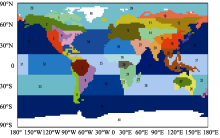
For more detail about the spatial distribution and variation of ff, we divided the globe into 40 geographical regions, including 29 land areas and 11 ocean areas (Fig. 1), based on previous work by TransCom-3 (Transport Comparation) ( Gurney et al., 2002). The emis-sion data used in this study were at a spatial resolution of 2° latitude × 2.5° longitude, so for each month we obtained an emission data matrix: FF [144, 91]. The training data matrix' FFTrain [144, 91, 360]'was needed to forecast the ff in 2009 with the Elman neural network. The third dimension of the FFTrain matrix denoted the time of the emissions from 1979 to 2008 (360 months). Theoretically, 13104 (144 × 91) neural networks needed to be built and trained. However, the ff mostly happened in densely populated areas on land. Therefore, FF was a sparse matrix. According to the divided regions in Fig. 1, we only needed to set up 29 Elman neural networks assuming that the grid ff in the same region evolved in a similar pattern.
 | Figure 1 The geographical locations of 40 regions divided according to TransCom-3 study. Locations 1-28 represent land areas: 1. Canadian tundra; 2. North America (NA) boreal forest; 3. Western US/Mexico; 4. Central NA agriculture; 5. NA mixed forest; 6. Central America and Caribbean; 7. South America (SA) rain forest; 8. SA coast and mountains; 9. SA wooded grasslands; 10. Eurasian tundra; 11. Eurasian boreal coniferous forest; 12. Eurasian boreal deciduous forest; 13. South and Central Europe; 14. Central Asian grasslands; 15. Central Asian desert; 16. East Asia mainland; 17. Japan; 18. Northern African desert; 19. Northern African grasslands; 20. Africa tropical forest; 21. Southern African grasslands; 22. Southern African desert; 23 Middle East; 24. India and bordering countries; 25. Maritime Asia; 26. Australian forest/grasslands; 27. Australian desert; 28. New Zealand. Locations 29-39 represent ocean areas: 29. Arctic Ocean; 30. North Pacific; 31. Tropical West Pacific; 32. Tropical East Pacific; 33. South Pacific; 34. North Atlantic; 35. Tropical Atlantic; 36. South Atlantic; 37. Tropical Indian Ocean; 38. Southern Indian Ocean; 39. Antarctic Ocean. Location 40 represents remote islands and ice caps. |
GEOS-Chem is a global 3D chemical transport model of atmospheric composition driven by assimilated meteorological observations from the Goddard Earth Observing System (GEOS) of the National Aeronautics and Space Administration (NASA) Global Modeling and Assimilation Office (GMAO) ( Feng et al., 2009, 2011). We used the model (v9-01-02) to relate prescribed ff predicted by the Elman neural network to atmospheric CO2 concentrations. The model was integrated with GEOS-5 meteorology for five years (2004-2008) from an initial condition of uniform CO2 (375.0 ppmv) as a 'spin up' period ( Nassar et al., 2010). The sources (or sinks) for the simulations in this study included emissions from fossil-fuel burning and cement production, biomass burning, biofuel burning, balanced biosphere (net ecosystem production), ocean, net terrestrial exchange, aircraft, and marine. We simulated CO2 concentrations in 2009 with two different sets of ff inventories as a prior input flux at a resolution of 2° latitude × 2.5° longitude: one was the real ff, and the other was forecasted by the Elman neural network (ENN ff) in 2009. We then compared the simulations with CO2 observations from the GlOBALVIEW dataset.
GLOBALVIEW-CO2 is a product of the Cooperative Atmospheric Data Integration Project maintained by the Carbon Cycle Greenhouse Gases Group of the National Oceanic and Atmospheric Administration, Earth System Research Laboratory (NOAA ESRL) ( Masarie et al., 2001). The data records are derived using data assimilation techniques based on different kinds of atmospheric measurements, such as in situ eddy covariance flux observation towers, air flask sampling, and marine and aircraft observations. We chose 56 observation sites in different latitudes from GLOBALVIEW-CO2 to estimate the ENN flux and to evaluate the resulting simulated atmospheric CO2 concentrations. GLOBALVIEW provided 48 pseudo-weekly CO2 data records per year. The chosen observation sites all adopted air flask sampling to measure CO2, which carries a smaller level of uncertainty than other kinds of data records from GLOBALVIEW.
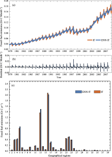
We used monthly averaged fossil-fuel CO2 emissions (1979-2008) as training data to build the Elman neural networks based on unequal geographical regions, as shown in Fig. 1. For instance, Fig. 2a shows the training process in region 16 (East Asian mainland). The network captured both the annual growth trend and the seasonal cycle well. In addition, the interdecadal variation from the late 1990s to 2003 transformed the increasing trend to a 'gentle' status, and the network successfully captured this characteristic. Accordingly, the residuals between the original ff and the computed emissions from ENN ff increased slightly during this period (Fig. 2b), where the residuals mainly depended on the amplitude of the variations of the monthly ff. Overall, the ff in region 16 maintained an increasing rate of ~ 3 Tg C yr-1 (1 Tg C = 1012 g C) from 1979 to 1997, and turned into an equilibrium trend between 1997 and 2003, then returned to a higher increasing rate of ~ 10 Tg C yr-1.
Similarly, 29 different Elman neural networks based on geographical regions where ff occurred were built and trained. We used these networks to forecast the grid emissions in 2009. The spatial distribution of the annual emissions in 2009 is shown in Fig. 2c. The total emissions were 8.0295 Gt C in 2009. East Asia (region 16 in Fig. 1), Europe (region 13), and North America (region 5) together accounted for more than half of the total emissions, with 25%, 17%, and 10% contribution (Fig. 2c), respectively. The total emissions in 2009 forecasted by the Elman networks were 8.2682 Gt C, which was 2.9% higher than the actual emissions. Considering that the uncertainty of the original emission data was 6%-7% according to previous research ( Andres et al., 1996, 2011), the performance of the networks was excellent. In addition, the difference between ff and ENN ff suggested an interannual variation trend, because the Elman network was theoretically based on the dynamic tendency of the historical data. For example, the two emissions for region 16 were 2.0718 Gt C (ff) and 2.0417 Gt C (ENN ff), which indicated a higher growth rate for 2009 compared with the last few years. Similarly, the emissions for region 13 (south and central Europe) likely increased with a slower rate during 2009 than before.
 | Figure 2 (a) Training process of the Elman neural network for region 16. The orange line denotes the original fossil-fuel emissions (ff) for region 16, and the blue line represents the trained emissions with the Elman neural network. (b) The distribution of residuals between original and trained ff for 1979 to 2008. (c) Total annual ff of different geographical regions in 2009. The number of the region is the same as in Fig. 1. The orange bars denote the results based on original data, and the blue bars are the emissions forecasted by the Elman neural networks. |
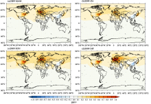
The ff inventories at different resolutions have been widely used for simulating CO2 concentrations or inverse modeling as an input flux ( Gurney et al., 2002; Nassar et al., 2010; Feng et al., 2011). Therefore, to evaluate the performance of the ensemble Elman neural networks, we conducted two simulations with distinct ff inventories (ff and ENN ff). These two simulations were identical in all other respects, including initial conditions and other input fluxes. Figure 3 shows the average seasonal difference (ENN ff - ff) between the two simulations. Overall, the difference between the two simulations was within ±1 ppmv globally, and was distributed mainly among Europe, North America, and East Asia, which was in accordance with the pattern shown in Fig. 2c. For the spatial distribution of sim-ulated CO2 concentration, the two simulated results were consi-stent with an acceptable difference. The global mean differences were: 0.082 ppmv for spring (March, April, and May (MAM)); 0.089 ppmv for summer (June, July, and August (JJA)); 0.125 ppmv for autumn (September, Octo-ber, and November (SON)); and 0.089 ppmv for winter (December, January, and February (DJF)). The division of the seasons is that for the Northern Hemisphere.
 | Figure 3 Comparison of seasonal averaged surface level CO2 in 2009 from a simulation using the original ff and another simulation using ENN ff. The difference is calculated by (ENN ff)-ff. The two simulations began with the same initial conditions and were identical in all other respects. |
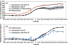
We examined the north-south gradient of CO2 concentrations with measurements from GLOBALVIEW, and compared it with the two simulations as mentioned above. The gradient was investigated through observations of CO2 concentration at different latitudes, and as for the simulations, we sampled the nearest grid to represent the observational site. Figure 4 shows the annual average pat-tern of the observations and simulations. The atmospheric CO2 concentration near the surface increased by about 3 ppmv from ~ 384 ppmv in the Southern Hemisphere to ~ 387 ppmv in the Northern Hemisphere. A sim-ilar pattern was found in the modeling results. However, the CO2 concentrations simulated by GEOS-Chem were ~ 1-2 ppmv higher than the observations, which is likely due to the missing processes in the model. The two simulations appeared to have an almost identical variation in different latitudes. In addition, the annual average standard variation representing the amplitude of the seasonal cycle is shown in Fig. 4b. The gradient was about 5 ppmv, which was induced by the influence of human activities and biological metabolism.
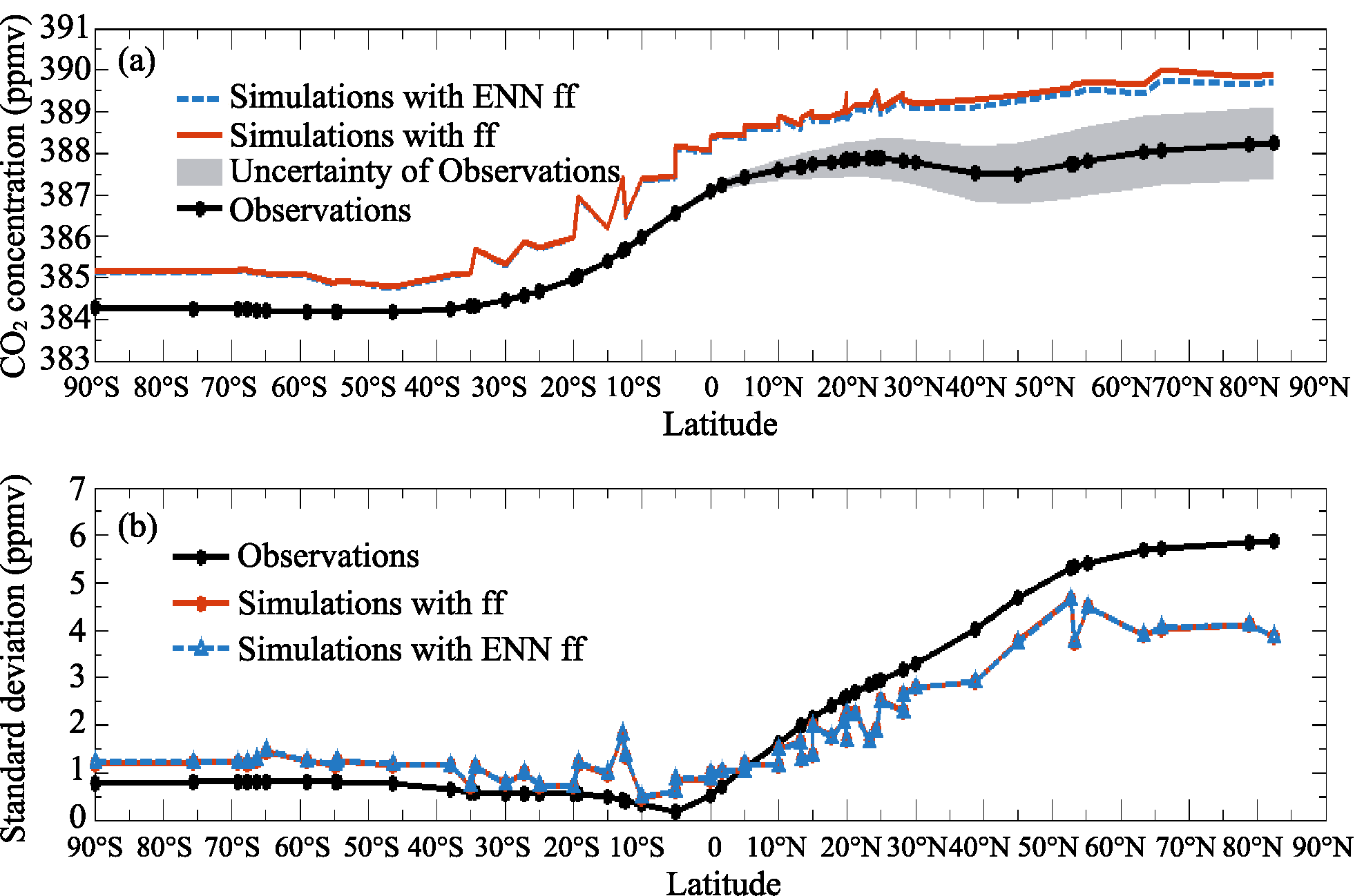 | Figure 4 (a) The observed and simulated annual mean CO2 concentrations near the surface at different latitudes during 2009. The observations are from GLOBALVIEW data products. Black dots denote the locations of the observation sites. Shading represents the standard deviations of the observations. (b) The standard deviation of annual average CO2 concentrations at different latitudes in 2009. The dots (red and black) and triangles denote the locations of observation sites, as in (a). |
The aim of this study was to develop an ensemble of Elman neural networks to forecast the spatial and temporal distribution of ff. We built and trained the networks based on the current grid emission data from 1979 to 2008. The results showed that the networks captured the primary aspects of the temporal variation of ff, which was better than conventional fitting methods. We also applied the forecasted emissions in 2009 to a global chemical transport model (GEOS-Chem) to comprehensively verify the predictions. The biases of the two simulations separately with ff and ENN ff ranged from -1 ppmv to +1 ppmv. A similar pattern emerged for the observed and simulated gradients, with a difference of less than 1 ppmv. Overall, the Elman neural network is potentially a useful tool for forecasting ff. At the same time, the predictions are valuable for modeling atmospheric CO2concentrations. In the future, we will carry on exploring the performance of other CO2 emissions forecasted with the method descr-ibed in this study.
Acknowledgments. This study was supported by the Strategic Priority Research Program'Climate Change: Carbon Budget and Relevant Issues of the Chinese Academy of Sciences (Grant No. XDA05040000) and the National Natural Science Foundation of China (Grant Nos. 41005023 and 41275046). The two anonymous reviewers are thanked for their helpful comments and suggestions.
| 1 |
|
| 2 |
|
| 3 |
|
| 4 |
|
| 5 |
|
| 6 |
|
| 8 |
|
| 9 |
|
| 10 |
|
| 11 |
|
| 12 |
|
| 13 |
|
| 14 |
|
| 15 |
|
| 16 |
|
| 17 |
|
| 18 |
|
| 19 |
|
| 20 |
|