

The Spatial Patterns of Initial Errors Related to the 'Winter Predictability Barrier' of the Indian Ocean Dipole
[FENG Rong1, 2 , DUAN Wan-Suo1, *  ]
]
]
|
|


In this study, using the Geophysical Fluid Dynamics Laboratory Climate Model version 2p1 (GFDL CM2p1) coupled model, the winter predictability barrier (WPB) is found to exist in the model not only in the growing phase but also the decaying phase of positive Indian Ocean dipole (IOD) events due to the effect of initial errors. In particular, the WPB is stronger in the growing phase than in the decaying phase. These results indicate that initial errors can cause the WPB. The dominant patterns of the initial errors that cause the occurrence of the WPB often present an eastern-western dipole both in the surface and subsurface temperature components. These initial errors tend to concentrate in a few areas, and these areas may represent the sensitive areas of the predictions of positive IOD events. By increasing observations over these areas and eliminating initial errors here, the WPB phenomenon may be largely weakened and the forecast skill greatly improved.
The Indian Ocean dipole (IOD) is an important ocean- atmosphere coupled phenomenon of interannual timescale in the tropical Indian Ocean ( Saji et al., 1999; Webster et al., 1999; Li et al., 2003). Whether or not it is independent of El Niño-Southern Oscillation (ENSO) is the subject of much debate ( Saji et al., 1999; Webster et al., 1999; Li et al., 2003; Behera et al., 2006; Ding and Li, 2012). Positive IOD events show positive sea surface temperature anomalies (SSTAs) in the western Indian Ocean, and negative SSTAs in the eastern Indian Ocean, along with strong easterly winds at the equator ( Saji et al., 1999; Webster et al., 1999; Li et al., 2002, 2003). Positive IOD events often bring large amounts of rain to east Africa, and drought to Indonesia and Australia ( Birkett et al., 1999; Black et al., 2003). It also has a close link with the monsoon and could affect global climate by Rossby waves ( Black et al., 2003; Annamalai and Murtugudde,2004). Negative IOD events present opposite SSTA patterns and climate effects. The strength of IOD events is usually measured by the IOD index ( Saji et al., 1999), which is the difference in SSTA between the western Indian Ocean (10°S-10°N, 50-70°E) and southeastern Indian Ocean (10°S-0°, 90-110°E). When the IOD index exceeds 0.5 standard deviation for three months, an IOD event occurs ( Song et al., 2007). Phase locking is an important characteristic of IOD events, and their occurrence, peak and decay are often phased-locked to the seasonal cycle ( Saji et al., 1999; Webster et al., 1999; Li et al., 2002, 2003; Behera et al., 2006). Positive IOD events often reverse the sign of the IOD index from negative to positive during the winter (January-March) preceding the IOD year, then peak in September and October in the IOD year, and finally reverse the sign again in the following winter not only in model outputs but also in reanalysis project data ( Wajsowicz, 2004).
As IOD events have significant climate effects not only in local regions but also around the world, many studies focus on its predictability ( Wajsowicz, 2004, 2005, 2007; Luo et al., 2007). Wajsowicz (2004, 2005, 2007) analyzed the predictability of SSTAs related to IOD events, and pointed out that a 'winter persistence barrier' exists in IOD events. Luo et al. (2007) computed the anomaly correlation coefficients (ACCs) of IOD index between observations and the Scale Interaction Experiment-Frontier Research Center for Global Change (SINTEX-F) model predictions, and found that the ACCs drop quickly across winter, indicating the existence of a 'winter predictability barrier' (WPB). As IOD events usually occur and decay in winter, the existence of the WPB, which indicates a rapid drop in forecast skill in winter, will cause the forecast of the occurrence and decay of IOD events to fail, as well as the appearance and disappearance of large-scale climate effects related to them, leading to great socioeconomic losses.
Prediction errors are usually caused by initial errors and model errors. In this study, we assume that the model is perfect and the prediction errors are only caused by initial errors. Based on this hypothesis, we try to determine whether the WPB exists in the Geophysical Fluid Dynamics Laboratory Climate Model version 2p1 (GFDL CM2p1) model, and what kind of initial errors result in the WPB. Discussion is made regarding the different development phases of IOD events, and initial errors related to the WPB are analyzed.
The remainder of the paper is organized as follows. The model is described in section 2. The experimental strategy and the characteristics of initial errors selected are described in section 3. And finally, a summary and discussion are presented in section 4.
The model used in this study is the GFDL CM2p1 coupled climate model, which contains an ocean model, an atmospheric model, a land model, and a sea ice model. It uses the Modular Ocean Model (MOM) 4p1 released in December 2009 as its ocean model, instead of the MOM4.0 used in the CM2.1 version. Scientists have confirmed that the climate simulations in the two versions are compatible. We introduce some basic characteristics of the coupled model below, but for more details readers may refer to Griffies (2009) as well as published papers on the CM2.1 model, such as Delworth et al. (2006) and Stouffer et al. (2006).
The ocean component of the coupled model is the MOM, which is a numerical representation of the ocean's hydrostatic primitive equations. Its horizontal resolution is 1° × 1° in most regions, and the meridional resolution reduces to (1/3)° near the equator. It has 50 vertical levels with a 10-m resolution in the upper 225 m. The atmospheric component of the model has a resolution of 2° latitude by 2.5° longitude with 24 levels in the vertical direction. The components of the coupled model are coupled though the GFDL's Flexible Modeling System (FMS; http://www.gfdl.noaa.gov/fms) and exchange fluxes every 2 h.
Song et al. (2007) assessed the simulation capability of the GFDL CM2.1 coupled model with respect to the seasonal cycle in the Indian Ocean from the aspects of surface winds, thermocline depth, SST, and precipitation by comparing model results with observations. They also focused on simulations of IOD events, and found that the CM2.1 coupled model successfully reproduces the basic characteristics of IOD events and its relation with ENSO. The GFDL CM2p1 model we use is the new version of the CM2.1 coupled model, and its simulations are consistent with the results in Song et al. (2007). That is, the IOD events in the GFDL CM2p1 are like the observed ones, which convince us to study IOD events with the GFDL CM2p1 model.
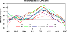
We run the GFDL CM2p1 model for 150 years with the forcing of 1990 values of aerosols, land cover, tracer gases, and insolation. The last 100 years are analyzed to eliminate the effect of initial adjustment processes. Given the higher intensity and more serious climate effects of positive IOD events compared with negative ones ( Black et al., 2003; Annamalai and Murtugudde, 2004), 10 of 26 positive IOD events are randomly chosen and analyzed in this study. Figure 1 shows the IOD indexes of the 10 IOD events. It is clear that most IOD events occur in the winter preceding the IOD year, and decay in the following winter, which is consistent with observations ( Wajsowicz, 2004).
 | Figure 1 The IOD indexes of 10 positive IOD events used in our study. E1-E10 denote the 10 IOD years in the model: 1, 3, 11, 20, 59, 81, 88, 90, 92, and 95. |
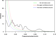
In this study, the model is assumed to be perfect, and thus prediction errors are only caused by initial errors. For convenience, we only superimpose different initial errors on temperatures at the sea surface and at the 95-m depth of the 'true state' for IOD events. The mean thermocline depth in the tropical Indian Ocean is about 110-125 m in the model, so the temperature anomalies at the 95-m depth can to a certain extent reflect the variety of the thermocline depth. Besides, the SST is an important variable closely connecting the ocean and the atmosphere. We believe that initial errors of those two variables could largely reflect the effects of temperature perturbations on the predictability of IOD events. The model IOD has a dominant period of about four years (Fig. 2). For the SSTA and 95-m depth temperature anomaly patterns in every other month of the four years preceding each IOD year, we scale them to yield the initial uncertainties. Thus, we have 24 pairs of initial errors after adjusting them to the same magnitude. Then, we superimpose those initial errors on IOD events and integrate them for 12 months from six different start months, with integrations starting from 7(-1) (where -1 signifies the year preceding the IOD year), 10(-1) and 1(0) (where 0 signifies the IOD year) across the winter in the growing phase of IOD events, and integrations starting from 4(0), 7(0), and 10(0) across the winter in the decaying phase of IOD events (Feng et al., 2014).
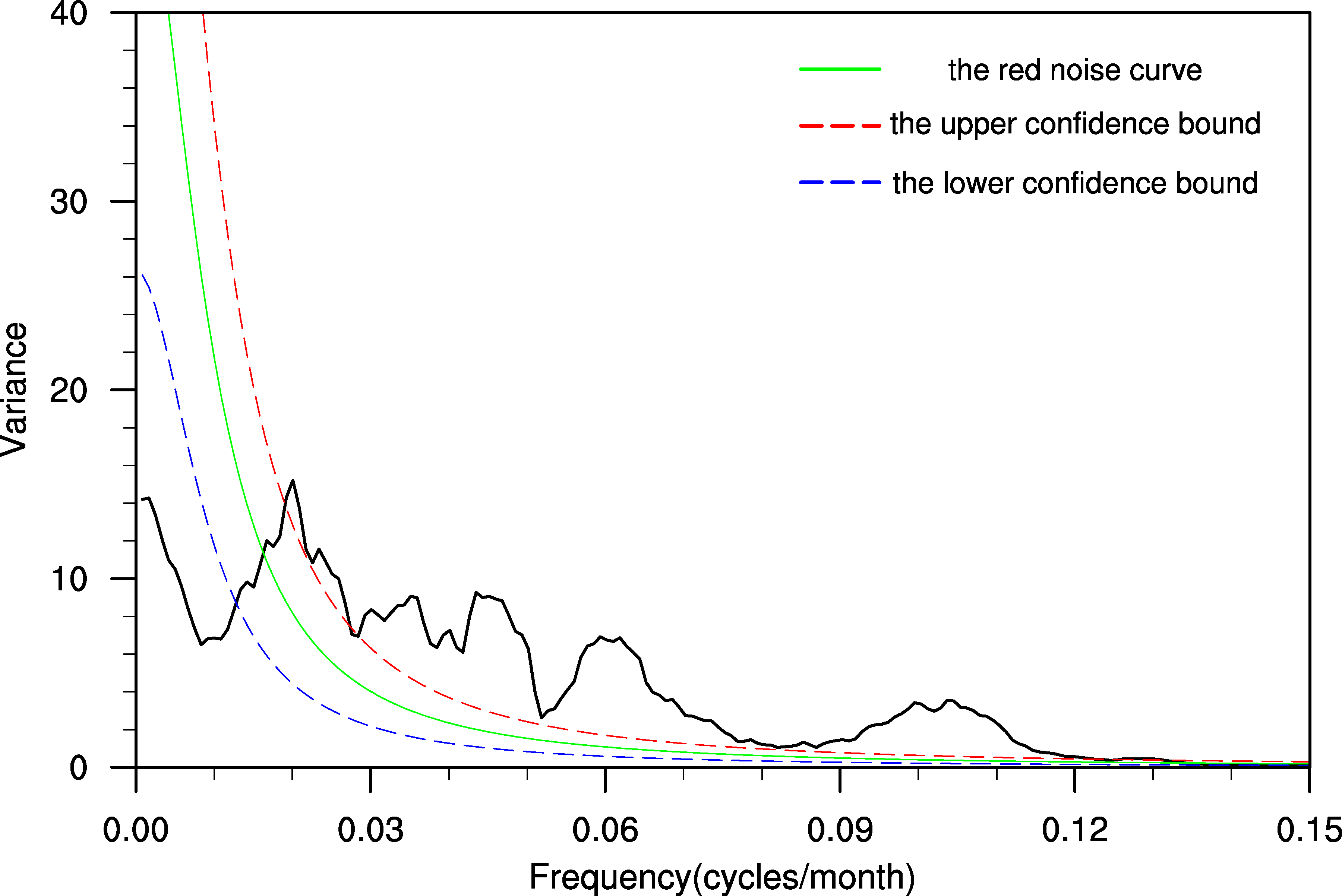 | Figure 2 Power spectrum of IOD index from 100-yr model data. The red and blue lines depict the significant intervals at the 0.05 level. |
The detailed steps are as follows. We denote the initial SSTAs and temperature anomalies at the 95-m depth as T1 and T2, with T1 ij and T2 ij representing values of T1 and T2at the grid ( i, j) in the Indian ocean, which ranges from 45°E to 115°E in longitude and 10°S to 10°N in latitude. T1 and T2are then scaled to the same magnitude by T10 = T1/ δ1 and T20 = T2/ δ2 with appropriate fractions 1/ δ1 and 1/ δ2 (where δ1 and δ2 represent positive numbers), respectively. T10 and T20 are initial errors superimposed on the initial states of the perfect IOD events. The norms
Before we try to find initial errors that cause the WPB of positive IOD events, and analyze their common characteristics, it is necessary to make sure that the WPB phenomenon mentioned in Luo et al. (2007) also exists in the GFDL CM2p1 model. Therefore, we perform the ACC analysis between 'observations' and 'predictions' as in Luo et al. (2007). The IOD index of the initial 10 positive IOD events are seen as 'observations'; the IOD index predicted after randomly superimposing four pairs of the aforementioned initial errors on each of the 10 positive IOD events for each start month are supposed as their corresponding 'predictions'. After the five-month running mean of the IOD index, which removes the effect of intraseasonal signals, the ACCs between the IOD index of 'observations' and that of 'predictions' are calculated for the six start months in Fig. 3. It is apparent that, no matter what the start month, the ACCs drop quickly across boreal winter in the growing phase of positive IOD events, which indicates the occurrence of WPB. Similarly, the WPB also exists in the decaying phase; particularly, the WPB is stronger in the growing phase than in the decaying phase. As uncertainties are only superimposed on temperatures of two levels in the ocean model, it indicates that initial errors can cause the WPB, and that initial errors in the ocean are highly influential in the development of IOD events, which inspires us to explore the sensitive areas of IOD events from the ocean temperature in future work.
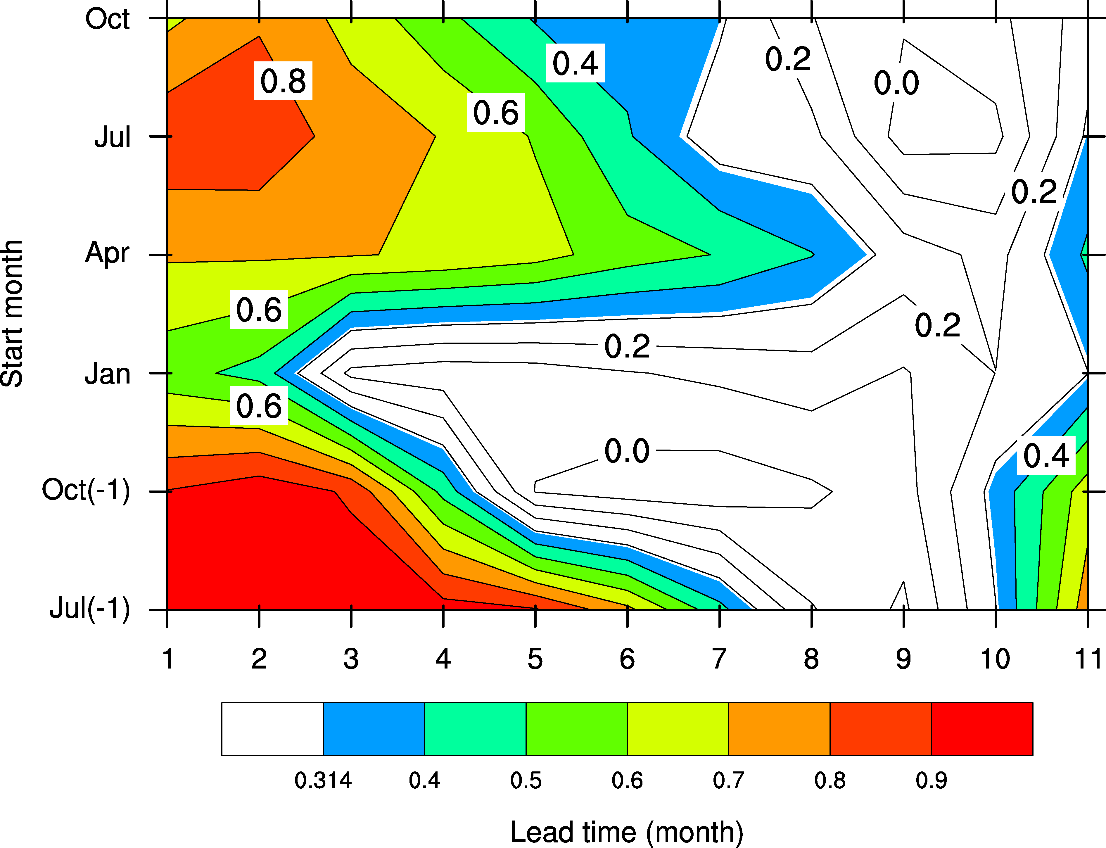 | Figure 3 The anomaly correlation coefficients (ACCs) between IOD index of 10 positive IOD events and that of predicted IOD events with initial errors superimposed for different start months and lead times. The contour interval is 0.1. The five-month running mean is used to remove the effect of the intraseasonal timescale. The ACCs significant at 0.05 level are colored. |
As the WPB exists in the GFDL CM2p1 model, we choose and analyze initial errors that cause the occurrence of WPB. The WPB means that the growth of prediction errors is fastest in winter. The prediction error is written as
We apply Combined Empirical Orthogonal Functions (CEOF) analysis to all pairs of SSTAs and temperature anomalies at the 95-m depth chosen to obtain the dominant pattern of initial errors for each start month. The CEOF1 for different start months are shown in Fig. 4. It is apparent that, for the start months of 7(-1), 4(0), 7(0), and 10(0), the surface and subsurface components of CEOF1 both display an eastern-western dipole, and the magnitude of anomalies in the subsurface is larger than that at the sea surface. Besides, the subsurface component of CEOF1 is very similar to the pattern of the peak positive IOD events, with one large anomaly locating at the southern branch of the western pole and the other large anomalies of opposite sign locating at the equator of the eastern Indian Ocean. However, the large values of the surface component locate diversely among different start months, with some locating in the middle of the south Indian Ocean, and some locating in the southeastern Indian Ocean. The CEOF1 with start months of 10(-1) and 1(0) are different from the above results: while the subsurface component shows an eastern-western dipole, the surface component displays a northwestern-southeastern dipole; besides, the large values of the subsurface component locate differently from the former four start months. Based on the above discussions, it is found that the dominant pattern of initial errors is an eastern-western
 | Figure 4 Left column: the surface component of CEOF1 for initial errors that cause the WPB with start months of (a) 7(-1), (c) 10(-1), (e) 1(0), (g) 4(0), (i) 7(0), and (k) 10(0). Right column: the subsurface component of CEOF1 for the corresponding start month (units: °C). |
dipole, both in the surface and subsurface components for most start months, and the large values tend to concentrate in a few areas. It is plausible that, if the initial errors in these few areas are removed, then the prediction errors of IOD events will be largely reduced and the predictive skill of IOD events will be greatly improved. Therefore, these areas may represent the sensitive areas of predictions of positive IOD events.
The IOD is an important ocean-atmosphere coupled phenomenon, which has a great effect on global climate. In this study, using the GFDL CM2p1 coupled model, we found that the WPB exists in the model not only in the growing phase but also the decaying phase of IOD events with initial errors superimposed, and the WPB is stronger in the growing phase. These results indicate that initial errors can cause the WPB. We applied CEOF analysis to initial errors that cause a significant WPB for different start months, and the dominant patterns of those initial errors show an eastern-wes-tern dipole both in the surface and subsurface temperature components for most start months. Such patterns of initial errors look like the sea temperature component of the mature phase of IOD events. It is therefore assumed that the prediction errors caused by the initial errors may have a dynamical mechanism similar to IOD events themselves. This, in any case, can be further explored by studying the similarities between initial anomaly patterns that most likely develop into an IOD event and the initial errors that have the largest effect on prediction uncertainties of IOD events.
Based on the above discussions, we found that initial errors with dipole patterns are inclined to cause the largest growth rate of prediction errors in winter, resulting in the occurrence of the WPB. These initial errors tend to concentrate in a few areas, and these areas may represent the sensitive areas of IOD prediction, which of course should be further confirmed by numerical experiments. In addition, we know that model errors may also influence the prediction uncertainties of IOD events. Therefore, how model errors influence the prediction uncertainties may be another key avenue of research for the predictability of IOD events, and should be investigated in depth in future studies. Also, what are the roles of thermodynamics and temperature advection in the rapid growth of prediction errors in winter? Many previous studies point out that ENSO has an important effect on the development of IOD events ( Ding and Li, 2012), and so how might ENSO affect the WPB? We will also try to address these questions in future work.
Acknowledgments. This work was jointly sponsored by the National Basic Research Program of China (Grant No. 2012CB955202) and the National Public Benefit (Meteorology) Research Foundation of China (Grant No. GYHY201306018).
| 1 |
|
| 2 |
|
| 3 |
|
| 4 |
|
| 5 |
|
| 6 |
|
| 7 |
|
| 9 |
|
| 10 |
|
| 11 |
|
| 12 |
|
| 13 |
|
| 14 |
|
| 15 |
|
| 16 |
|
| 17 |
|
| 18 |
|
| 19 |
|