Since the mid-20th century, the decadal variation of sea surface temperature (SST) in the northern Indian Ocean (NIO) has been characterized by a consistent warming trend. The warming is regarded as a forcing agent driving the interdecadal variability of East Asian summer monsoon (EASM) ( Li et al., 2008; Zhou et al., 2008; Li et al., 2010a). Moreover, the Indian Ocean warming could cause the North Pacific storm track and North Atlantic storm track to shift northward, and force the annular trend in both hemispheres through interactions between forced stationary wave anomalies and transient eddies ( Li et al., 2010b; Chu et al., 2013).

The attribution of this basin-wide Indian Ocean warming has been investigated in several studies. Through analyzing the Coupled Model Intercomparison Project Phase 5 (CMIP5) models, Dong and Zhou (2014) suggested that the Indian Ocean SST warming is the competing result of the warming effect of GHGs (Greenhouse Gases) with the cooling effect of aerosols. Barnett et al. (2005) also pointed out that the surface heat budget over the Indian Ocean is the result of a cancellation between the warming background of GHGs and the cooling effect of sulfate aerosol. Besides the surface heat budget, the role of oceanic dynamic processes in inducing the warming has also been explored ( Alory and Meyers, 2009; Rao et al., 2012). These authors attribute the Indian Ocean warming to the decreasing trend in upwelling-related oceanic cooling. Alory and Meyers (2009) also suggested that the surface shortwave flux, which is affected by aerosols, acts as a damping term to decelerate the warming rate.

Unlike the aforementioned investigations, our study emphasizes the role of aerosols rather than GHGs and ocean dynamics. The role of the aerosol effect in NIO warming simulated by CMIP5 models is of special interest to us for several reasons. Firstly, the role of aerosols in modulating the sea surface heat budget and SST is important and has been widely studied. For instance, the 20th-century climate variability of North Atlantic SST may have been primarily driven by increasing aerosol emissions, which reduced the shortwave radiation reaching the ocean surface through the aerosol direct, and especially indirect, effects ( Booth et al., 2012). Anthropogenic aerosols also have impacts on trends of the sub-thermocline temperature of the southern Indian Ocean through altering the ocean circulations ( Cowan et al., 2013). The cooling effect of aerosols on the NIO contributes to the weakening of the meridional gradient of SST in the NIO during summer, thus changing the monsoon rainfall in India and the Sahel ( Chung and Ramanathan, 2006). Using a slab ocean model, Ganguly et al. (2012) also indicated that anthropogenic aerosols could reduce the SST in the NIO, thus weakening the meridional SST gradient, which is crucial for monsoon circulation, and resulting in a decrease of summer monsoon rainfall over South Asia.

Secondly, there are more models considering the aerosol indirect effect (AIE) to represent the aerosol effect on climate in CMIP5. The behavior of these CMIP5 models in simulating the basin-wide Indian Ocean warming and the role of AIE in NIO warming simulation are not well documented. Furthermore, there are still large uncertainties in the AIE representation of climate models. For example, models may overestimate the lifetime cycle of sulfate aerosols in clouds, resulting in overestimation of the direct and indirect effect of sulfate aerosols ( Harris, 2013). Using a multiscale modeling framework model, Wang et al. (2011) found that there is an overestimation of the AIE simulated by conventional global climate models. Moreover, uncertainties in the subgrid cloud parameterization can propagate into the scheme for aerosol-cloud interaction ( Golaz et al., 2011). Therefore, it is necessary to study the aerosol effect on SST, especially the AIE, produced by various models in CMIP5.

As seen from the emission dataset used in CMIP5, recommended by the Fifth Assessment Report of the Intergovernmental Panel on Climate Change (IPCC AR5), the anthropogenic aerosol emissions from the continent near the Indian Ocean has continued increasing since 1950, especially in South Asia ( Lamarque et al., 2010). Therefore, the NIO has become a region susceptible to the impact of anthropogenic aerosols. As the SST trend in the Indian Ocean is the result of competition between the cooling effect of aerosols and the warming effect of GHGs ( Dong and Zhou, 2014), whether or not models can reproduce the warming may rely on their ability to reasonably reproduce the aerosol cooling effect. As the AIE remained difficult to be modeled in IPCC AR5, this study attempts to compare the behaviors of seven representative CMIP5 models in simulating the NIO warming and, especially, the AIE on ocean warming.

Two CMIP5 experiments are used to analyze the Indian Ocean surface heat budget in this study. The first is the historical run with all the time-varying climate forcing agents such as GHGs, ozone, anthropogenic aerosols, and volcanic eruptions. Most analysis and evaluations are performed on this standard experiment. The other is the historical-AERO experiment, which is forced by changing aerosols only. The historical-AERO experiment is used to further prove our conclusion about the aerosol effect.

Among the CMIP5 models, we choose those that satisfy the criterion that both the historical and historical-AERO runs each have more than three ensemble realizations. Under this criterion, seven models (GFDL-CM3, CESM-CAM5.1-FV2, CSIRO-MK3-6-0, NorESM1-M, IPSL-CM5A-LR, CanESM2, and FGOALS-g2) are selected. Their descriptions for the treatment of the aerosol concentration specification and AIE are listed in Table 1. In addition, detailed information about the ensemble realization and the aerosol module of these models can be found in Ekman (2014).

The analysis is performed on the ensemble mean and the variables including total cloud fraction (CLDTOT), surface upward latent heat flux (LHFLX, changed to the downward direction in our study), surface upward sensible heat flux (SHFLX, changed to the downward direction in our study), surface downwelling longwave radiation (FLDS), surface upwelling longwave radiation (FLUS), surface downwelling shortwave radiation (FSDS), surface upwelling shortwave radiation (FSUS), surface downwelling clear-sky shortwave radiation (FSDSC), and SST. The observational SST data are from the Hadley Centre Sea Ice and Sea Surface Temperature Dataset (HadISST)( Rayner et al., 2003).

Table 1

Table 1

Table 1 Seven CMIP5 (Coupled Model Intercomparison Project Phase 5) models and descriptions of their treatment of aerosol emissions and the AIE (Aerosol Indirect Effect). For aerosol concentration, 'online' means that the aerosol concentration is prognostic and the emission source is specified in the model. 'Prescribed' represents that the aerosol concentration is prescribed using the output data from other aerosol models. For the first AIE, 'prognostic' means the cloud number concentration (CDNC) is prognostic based on an explicit aerosol activation scheme, such as Abdul-Razzak and Ghan (2000), while 'diagnostic' means the CDNC is based on the empirical relationship between aerosols and CDNC. 'Yes' or 'No' indicates whether or not the model considers the second AIE. Model Aerosol concentration 1st AIE 2nd AIE Reference GFDL-CM3 online prognostic Yes Donner et al. (2011) CSIRO-MK3-6-0 online diagnostic Yes Rotstayn et al. (2012) CESM-CAM5.1-FV2 online prognostic Yes Meehl et al. (2013) NorESM1-M prescribed prognostic Yes Kirkevaget al. (2013) IPSL-CM5A-LR prescribed diagnostic No Dufresne et al. (2013) CanESM2 online diagnostic No Gillett et al. (2012) FGOALS-g2 prescribed prognostic Yes Li et al. (2013) Note: GFDL-CM3 (Geophysical Fluid Dynamics Laboratory Climate Model, version 3); CSIRO-MK3-6-0 (Commonwealth Scientific and Industrial Research Organisation Mark, version 3.6.0); CESM-CAM5.1-FV2 (Community Earth System Model, Community Atmosphere model version 5.1, with Finite Volume dynamic core); NorESM1-M (Norwegian Earth System Model, version 1, mid resolution); IPSL-CM5A-LR (L'Institut Pierre-Simon Laplace Coupled Model, version 5A, coupled with the Nucleus for European Modelling of the Ocean (NEMO), low resolution); CanESM2 (Second Generation Canadian Earth System Model); FGOALS-g2 (The Flexible Global Ocean-Atmosphere-Land system model, Grid Version 2).

Table 1 Seven CMIP5 (Coupled Model Intercomparison Project Phase 5) models and descriptions of their treatment of aerosol emissions and the AIE (Aerosol Indirect Effect). For aerosol concentration, 'online' means that the aerosol concentration is prognostic and the emission source is specified in the model. 'Prescribed' represents that the aerosol concentration is prescribed using the output data from other aerosol models. For the first AIE, 'prognostic' means the cloud number concentration (CDNC) is prognostic based on an explicit aerosol activation scheme, such as Abdul-Razzak and Ghan (2000), while 'diagnostic' means the CDNC is based on the empirical relationship between aerosols and CDNC. 'Yes' or 'No' indicates whether or not the model considers the second AIE.

Since the traditional method of evaluating the strength of the AIE is not possible due to the unavailability of direct variables and experiments in these models, we need to define a metric to measure the strength of the AIE on the surface radiation budget. In this context, the word 'indirect' means that the AIE perturbs surface radiation using cloud as the media to take effect. Therefore, a variable reflecting the change of surface radiation in cloudy sky conditions may be an ideal choice for our metric.

In the models, FSDS is the sum of the weighed mean of FSDSC and the cloudy sky surface downwelling shortwave flux (FSDSCL) with the weight as the cloud amount. In CMIP5 data, we can only obtain CLDTOT, rather than cloud amount, in every layer. So, in approximation, we can deduce FSDSCL as Although FSDSCL could also be influenced by the aerosol direct effect, our analysis in the next section shows that the trend of FSDSCL can still be used as a metric to measure the indirect effect, because the aerosol direct effect plays a limited role in perturbing the NIO surface radiation budget.

The NIO here is defined as the oceanic area within (20°S-20°N, 50-90°E). The heat budget for the 0-50 m layer of this region is analyzed. We assume that 95% of the shortwave heat flux can be absorbed by the 0-50 m layer, as used in Alory and Meyers (2009).

All seven models consistently simulate the increasing trends of surface net longwave flux (FLNS) and SHFLX at the surface (Table 2), which is mainly caused by the atmospheric warming induced by increasing GHG emissions, consistent with other studies ( Barnett, 2005; Alory and Meyers, 2009). Both the increasing surface FLNS and SHFLX contribute to the SST warming. The decreasing trend of FSDS is also obvious in every model, implying that the decreasing trend of FSDS acts consistently among all models as the damping factor exerted on SST warming. The consistent FLNS and FSDS trends among these models prove that there is competition between the GHG warming effect and the aerosol cooling effect, consistent with the results of Dong and Zhou (2014). Meanwhile, the LHFLX trends are different in the seven models, being positive in GFDL-CM3, CSIRO-MK3-6-0, CESM-CAM5.1- FV2, and NorESM1-M, and negative in the remaining models.

Although every model produces an SST increasing trend, all their magnitudes of SST warming are less than the observed value of 0.63 K (50 yr)^-1. Here, we use 0.5 K (50 yr)^-1 as the criterion to evaluate the ability of the model to simulate the SST warming. Models that produce a higher than 0.5 K (50 yr)^-1 SST increasing trend are classified as better models, and vice versa. It is clear to see that those models simulating the SST increasing trend well (IPSL-CM5A-LR, CanESM2, and FGOALS-g2) produce less FSDS decreasing than others. The sum of FLNS, SHFLX, and LHFLX, which can be regarded as the heat flux to the ocean contributed by the atmosphere, except for solar radiation, contributes to the SST warming. However, the sum of these variables cannot explain well the differences of the SST trends among the models.

Further, the 0-50 m layer annual mean heat budgets over the NIO for all the models are shown in Fig. 1. It is clearer to see that, for all seven models, the decreasing of the surface net shortwave flux has the main damping effect on the increasing SST, which supports the conclusion of Alory and Meyers (2009). Because there is much less change of upward shortwave flux than that of FSDS, the decrease of FSDS becomes the main damping force. The characteristics of the latent heat flux and sensible heat flux trends are the same as shown in Table 2. There is no obvious and consistent trend for the advective and diffusive fluxes among the models, with a slight increasing trend for CESM-CAM5.1-FV2 and a slight decreasing trend for CSIRO-MK3-6-0, NorESM1-M, and FGOALS-g2.

The above analysis shows that the magnitude of the decreasing trend of FSDS may be the main factor affecting whether or not the model can produce the SST increasing trend to a satisfactory level, i.e., as compared to the observation. The trend of FSDS is mainly modulated by the changes of both aerosols and clouds. As the total cloud amount in the seven models shows no obvious trend (data not shown), the increasing aerosol emissions is the major contributor to the decrease of FSDS in the historical simulation ( Lamarque et al., 2010).

Table 2

Table 2

Table 2 Trends of annual mean surface net longwave flux (FLNS; positive for the downward direction; W m-2(50 yr)-1), sensible heat flux at surface (SHFLX; positive for the downward direction; W m-2(50 yr)-1), latent heat flux at the surface (LHFLX; positive for the downward direction; W m-2(50 yr)-1), surface downwelling shortwave flux (FSDS; W m-2(50 yr)-1), and SST (K (50 yr)-1)) averaged over the NIO during the period 1950-2000 for the historical experiment. ATM is the sum of FLNS, SHFLX, and LHFLX. Model FLNS SHFLX LHFLX ATM FSDS SST trend GFDL-CM3 1.87 0.59 3.56 6.02 -5.8 0.11 CSIRO-MK3-6-0 1.03 0.38 2.6 4.01 -3.68 0.25 CESM-CAM5.1-FV2 1.84 0.3 0.67 2.81 -4.22 0.34 NorESM1-M 1.78 0.58 0.95 3.31 -2.8 0.27 IPSL-CM5A-LR 3.01 0.75 -1.29 2.47 -2.21 0.58 CanESM2 1.54 0.63 -1.49 0.68 -0.52 0.54 FGOALS-g2 2.61 0.66 -0.53 2.74 -2.25 0.52 HadISST N/A N/A N/A N/A N/A 0.63 Note: HadISST (Hadley Centre Sea Ice and Sea Surface Temperature Dataset).

Table 2 Trends of annual mean surface net longwave flux (FLNS; positive for the downward direction; W m-2(50 yr)-1), sensible heat flux at surface (SHFLX; positive for the downward direction; W m-2(50 yr)-1), latent heat flux at the surface (LHFLX; positive for the downward direction; W m-2(50 yr)-1), surface downwelling shortwave flux (FSDS; W m-2(50 yr)-1), and SST (K (50 yr)-1)) averaged over the NIO during the period 1950-2000 for the historical experiment. ATM is the sum of FLNS, SHFLX, and LHFLX.

Figure 1

Figure Option ViewDownloadNew Window

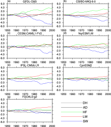
Figure 1 Comparison of the annual mean heat budgets in the 0-50 m layer over the NIO for different models from 1950 to 2000. Except for the derivative of the 0-50 m heat content, which shows absolute values, the data are presented as anomalies from the mean of the first five years for each series, and have been smoothed with a 9-yr running mean. Advective and diffusive fluxes are calculated as the closing term between the derivative of the annually averaged 0-50 m heat content (DH) and the surface fluxes. The surface fluxes include HF (sensible heat flux plus latent heat flux), SW (surface net shortwave flux), and LW (surface net longwave flux). All variables are in units of W m-2.

To study the aerosol effect on the FSDS decreasing trend, we list the FSDSCL and FSDSC trends of each model in Table 3. Models that fail to simulate the SST increasing trend produce a significantly stronger FSDSCL decreasing trend than other models. For example, in the standard historical simulation, the FSDSCL decreasing trend of GFDL-CM3 is the largest, reaching -6.23 W m^-2(50 yr)^-1, which greatly contributes to its FSDS decreasing trend of -5.8 W m^-2(50 yr)^-1. Thus, its corresponding SST increasing trend is only 0.11 K (50 yr)^-1, which is the lowest value among the models. Those models that fail to simulate the SST increasing trend also produce a larger magnitude of the FSDSCL decreasing trend in their corresponding historical-AERO simulations, agreeing with the result from the standard historical simulation. These results indicate that the strength of the AIE plays an important role in the model's ability to simulate the NIO warming. Actually, although the FSDSC decreasing trend of IPSL-CM5A-LR is the second largest among the models, due to its relatively weaker AIE characterized by its smaller FSDSCL decreasing trend and much lower total cloud amount, the model still produces the highest SST increasing trend.

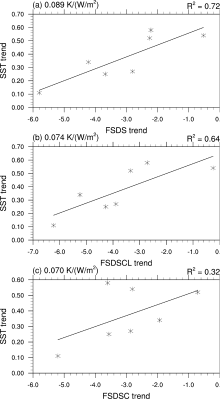
To show more clearly the importance of the FSDSCL trend in driving the SST warming, we regress the SST increasing trend on the FSDS trend (Fig. 2a), FSDSCL trend (Fig. 2b), and FSDSC trend (Fig. 2c). The stronger the decreasing trend of FDSCL is, the smaller the SST increasing trend. The regression coefficient pass the Student's t-test at the two-tailed 0.05 significance level and the squares of the correlation coefficient are also as high as 0.64, meaning the trend of FSDSCL, as a metric to measure the strength of the AIE, is an important contributing factor to the simulation of the NIO warming. In contrast, if we regress the SST increasing trend on FSDSC, the squares of the correlation coefficient are only 0.32 and do not pass the statistical test. It is clear that the regression of the SST trend on FSDS is more deterministic, with the highest squares of the correlation coefficient reaching 0.72. This is expected, because the FSDS trend exerts influence on the SST trend directly, and is caused by both the aerosol direct and indirect effects. If we regress the FSDS trend on the FSDSC trend and the FSDSCL trend respectively (data not shown), the FSDSCL trend can interpret 94% of the FSDS trend, while the FSDSC trend interprets only 24% of the FSDS trend. These results all indicate that the aerosol direct effect, by which FSDSC is mainly affected, has a limited effect on the FSDS and SST trends, whereas the AIE plays a more important role. This is consistent with the findings of Dong and Zhou (2014).

Table 3

Table 3

Table 3 Trends of annual mean clear-sky surface downwelling shortwave flux (FSDSC; W m-2(50 yr)-1), cloudy-sky downwelling shortwave radiation flux at the surface (FSDSCL; W m-2(50 yr)-1) and SST (K) averaged over the NIO during the period 1950-2000. FSDSCL-AERO is the trend for FSDSCL produced by the anthropogenic aerosols only forcing simulations (historical-AERO simulations). The total cloud amount (CLDTOT; %) is shown as the average value during the period, rather than the trend. Model FSDSC FSDSCL CLDTOT FSDSCL-AERO SST trend GFDL-CM3 -5.20 -6.23 71 -5.41 0.11 CSIRO-MK3-6-0 -3.56 -4.27 67 -3.77 0.25 CESM-CAM5.1-FV2 -1.93 -5.24 63 -3.41 0.34 NorESM1-M -2.86 -3.89 57 -4.99 0.27 IPSL-CM5A-LR -3.60 -2.72 45 -1.37 0.58 CanESM2 -2.81 -0.25 64 -2.16 0.54 FGOALS-g2 -0.70 -3.34 53 N/A 0.52

Table 3 Trends of annual mean clear-sky surface downwelling shortwave flux (FSDSC; W m-2(50 yr)-1), cloudy-sky downwelling shortwave radiation flux at the surface (FSDSCL; W m-2(50 yr)-1) and SST (K) averaged over the NIO during the period 1950-2000. FSDSCL-AERO is the trend for FSDSCL produced by the anthropogenic aerosols only forcing simulations (historical-AERO simulations). The total cloud amount (CLDTOT; %) is shown as the average value during the period, rather than the trend.

Figure 2

	Figure Option ViewDownloadNew Window
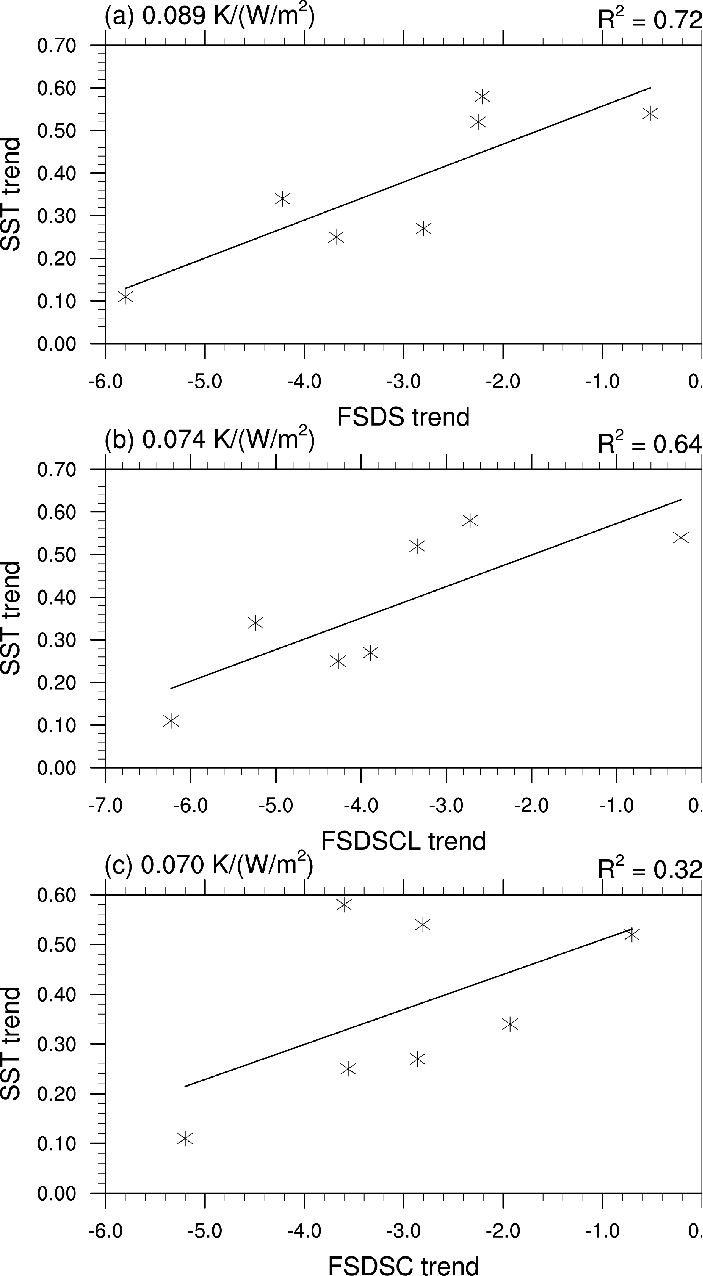	Figure 2 Scatter plot of the trends of SST ( y axis) vs. the trends of FSDS, FSDSCL, and FSDSC averaged over the NIO.

Overall, the heat budget analysis shows that the GHG- induced surface net longwave radiation flux change is the main contributing factor to increasing SST, whereas the FSDS decreasing trend is the main damping factor for ocean warming. Whether or not a model can simulate the NIO warming well depends on its simulation of the FSDS decreasing trend, which is affected more by the strength of the AIE, rather than the aerosol direct effect.

In this study, we chose seven CMIP5 models that simulate both the aerosol direct and indirect effects. The heat flux budgets of these models were compared in order to study the role of the aerosol cooling effect in the decadal-scale NIO warming. The results show that the increased GHGs from 1950 to 2000 contribute to the ocean warming, and the major damping factor is aerosols inducing the decrease of FSDS. This is consistent with the results of Barnett (2005) and Dong and Zhou (2014), indicating that the aerosol effect very likely offsets the GHG effect. Although the FSDS decreasing trend is driven by both the aerosol direct and indirect effect, our study shows that the AIE plays the more important role.

Those models that produce less of an FSDS decreasing trend (IPSL-CM5A-LR, CanESM2, and FGOALS-g2) simulate a relatively larger magnitude of the SST increasing trend, which is closer to observation. This can be attributed to their weaker AIE compared to the other models. On the contrary, those models with relatively stronger AIE (GFDL-CM3, CSIRO-MK3-6-0, CESM-CAM5.1- FV2, and NorESM1-M) fail to reproduce the SST increasing trend in a comparable fashion to that observed. From the data in Table 1, we can see that those models simulating the SST trend less successfully adopt a more sophisticated scheme for aerosol-cloud interaction. It has been pointed out previously that a more sophisticated scheme for aerosol-cloud interaction is likely to improve the representation of recent observed temperature trends in more regions than models that adopt a simpler scheme ( Ekman, 2014). However, our study indicates that, in the NIO, the AIE of these models may be too strong to reproduce a reasonable aerosol cooling effect and a realistic ocean warming. It should be noted that FGOALS-g2 also uses a relatively sophisticated scheme for aerosol-cloud interaction; however, it still produces a comparable-to- observed basin-wide Indian Ocean warming, which is believed to be as a result of the tuning of the strength of its AIE in its implementation ( Li et al., 2013).

Most of the models studied here do not simulate well the increasing trend of advective and diffusive heat flux into the 0-50 m layer over the NIO, which is inconsistent with the results of Alory and Meyers (2009). This inconsistency needs further investigation. As our defined metric still possesses uncertainty, it is also necessary to establish a more accurate metric for measuring the strength of the AIE.

Acknowledgments. We acknowledge the World Climate Research Programme's Working Group on Coupled Modelling, which is responsible for the CMIP, and we thank the climate modeling groups (listed in Table 1 of this paper) for producing and making available their model output. For CMIP, the U.S. Department of Energy's Program for Climate Model Diagnosis and Intercompar-ison provides coordinating support and leads the development of the software infrastructure in partnership with the Global Organization for Earth System Science Portals. We also appreciate the valuable suggestions from the two anonymous reviewers. This work was supported by Strategic Priority Research Program of the Chinese Academy of Sciences (Grant No. XDA05110304) and the National Basic Research Program of China (973 Project, Grant No. 2010CB951904).