

Application of a Derivative-Free Method with Projection Skill to Solve an Optimization Problem
[PENG Fei1, 2 , SUN Guo-Dong1, *  ]
]
]
|
|


Improving numerical forecasting skill in the atmospheric and oceanic sciences by solving optimization problems is an important issue. One such method is to compute the conditional nonlinear optimal perturbation (CNOP), which has been applied widely in predictability studies. In this study, the Differential Evolution (DE) algorithm, which is a derivative-free algorithm and has been applied to obtain CNOPs for exploring the uncertainty of terrestrial ecosystem processes, was employed to obtain the CNOPs for finite-dimensional optimization problems with ball constraint conditions using BurgersŌĆś equation. The aim was first to test if the CNOP calculated by the DE algorithm is similar to that computed by traditional optimization algorithms, such as the Spectral Projected Gradient (SPG2) algorithm. The second motive was to supply a possible route through which the CNOP approach can be applied in predictability studies in the atmospheric and oceanic sciences without obtaining a model adjoint system, or for optimization problems with non-differentiable cost functions. A projection skill was first explanted to the DE algorithm to calculate the CNOPs. To validate the algorithm, the SPG2 algorithm was also applied to obtain the CNOPs for the same optimization problems. The results showed that the CNOPs obtained by the DE algorithm were nearly the same as those obtained by the SPG2 algorithm in terms of their spatial distributions and nonlinear evolutions. The implication is that the DE algorithm could be employed to calculate the optimal values of optimization problems, especially for non-differentiable and nonlinear optimization problems associated with the atmospheric and oceanic sciences.
Nonlinear optimization problems (NOPs) are widely employed in the atmospheric and oceanic sciences; for instance, variational data assimilation, and sensitivity analysis of the model to initial and parameter conditions ( Ishikawa et al., 2001; Mu et al., 2004; Robert et al., 2006). Consequently, optimization approaches to solve NOPs play an important role in this field, and contribute to advancing progress in the predictability of atmospheric or oceanic systems, as well as improving the forecasting skill of numerical models ( Duan et al., 2014; Mu and Duan, 2003; Zheng et al., 2012b).
Some special approaches related to NOPs have been applied in atmospheric and oceanic studies. For example, the conditional nonlinear optimal perturbation (CNOP) approach is used to investigate predictability and uncertainty ( Mu and Duan, 2003; Mu et al., 2007; Yu et al., 2011), and variational data assimilation (VDA) is employed to find the optimal initial field in order to reduce initial errors in numerical models ( Ishikawa et al., 2001; Robert et al., 2006). As well as predictability problems related to initial errors, those related to parameter errors have also been investigated. For example, optimal estimates of model parameters can be obtained by fitting model results to observations ( Tziperman and Thacker, 1989; Wang et al., 2005). In addition, an optimal forcing vector approach is applied to correct model errors for improving the model simulation ability ( Duan et al., 2014). The above approaches have the potential to improve the forecasting skill and reduce uncertainty in numerical simulations. Traditional optimization algorithms, which require the derivatives of the cost functions, are most commonly employed during optimization processes of these approaches. However, when the derivatives do not exist or cannot be calculated, it is difficult to search for the optimal values using these traditional optimization algorithms, which limits their broad application. Consequently, derivative-free optimization approaches are receiving increasing attention in solving NOPs. They have been used in VDA ( Fang et al., 2009; Gratton et al., 2014; Zheng et al., 2012b) and for optimizing model parameters ( Severijns and Hazeleger, 2005; Wang and Huo, 2013), the results of which have demonstrated their efficiency. The indication is that derivative-free optimization algorithms are powerful and important tools for future research, and thus it is necessary to further explore their application, for instance in calculating CNOPs.
In fact, the CNOP, a nonlinear generalization of linear singular vectors (LSVs), is the optimal value of a nonlinear optimization problem. The CNOP approach was first proposed to find the optimal initial perturbation (CNOP-I)of a nonlinear system ( Mu et al., 2003). Its application was then extended to identify the combined optimal mode of the initial perturbation and model parameter perturbation (CNOP-I and CNOP-P) ( Mu et al., 2010). In short, a CNOP is a kind of initial perturbation or parameter perturbation with maximum nonlinear evolution at the prediction time and satisfying a given constraint. It has been applied to investigate the predictability of ENSO (including the optimal precursor, the effects of nonlinearity on error growth, and the importance of model parameter error to the spring predictability barrier) ( Duan and Mu, 2006; Duan et al., 2004; Mu and Duan, 2003; Mu and Wang, 2007; Yu et al., 2011), the nonlinear growth of instability of the oceanic thermohaline circulation ( Mu et al., 2004), the adaptive observations of typhoons ( Mu et al., 2009), the stability of a grass ecosystem ( Mu and Wang, 2007; Sun and Mu, 2009), and ensemble prediction ( Mu and Jiang, 2008). All these applications illustrate that the CNOP method is a useful tool for predictability and stability studies associated with the atmospheric and oceanic sciences. Because of its explicit physical meaning, the CNOP approach is expected to play an increasing role in weather and climate studies in the future.
Generally, during the maximization process to calculate CNOPs, the derivative-based traditional optimization algorithms, such as the sequential quadratic programming algorithm ( SQP, Barclay et al., 1998), the spectral projected gradient algorithm ( SPG2, Birgin et al., 2000), and the limited memory Broyden-Fletcher-Goldfarb-Shanno algorithm ( L-BFGS, Liu and Nocedal, 1989), are applied and the adjoint system is always used to determine the gradients of the cost functions. However, not all numerical models have available adjoint systems, which limits the broad application of the CNOP approach. In addition, if the cost functions are non-differentiable, these derivative-based optimization approaches cannot be used. Consequently, it is necessary to explore a derivative-free optimization algorithm for calculating CNOPs. For example, Zheng et al. (2012a) applied a genetic algorithm (GA) to get CNOPs and discussed the predictability problems related to ŌĆ£on-offŌĆØ switches. They stated that the GA was more powerful in determining the optimal values than the traditional algorithm. Recently, a derivative-free global optimization approach, the Differential Evolution (DE) algorithm, has been employed to obtain the CNOP-Ps satisfying box constraint conditions by using a dynamic global vegetation model with intermediate complexity ( Sun and Mu, 2012, 2013). However, this algorithm was just employed to obtain the CNOP in a lower dimensional optimization problem related to terrestrial ecosystem processes. Furthermore, it has not yet been used to deal with a ball constraint for a finite-dimensional optimization problem, which is important in the CNOP approach.
In this study, a projection skill, which is also employed in some traditional optimization algorithms for solving optimization problems with ball constraint conditions, such as the SPG2 algorithm, was explanted to the DE algorithm for calculating the CNOP of the finite-dimensional NOP with a ball constraint condition. The CNOP can be associated with the initial or parameter perturbations; but here, the CNOP related to initial perturbations was computed. To test the validity of the DE algorithm and apply the DE algorithm in a discussion of the predictability of the atmosphere and ocean, a comparison was made using the DE algorithm and the traditional algorithm. Specifically, the DE and SPG2 algorithms were both employed to obtain the CNOPs of the NOPs with ball constraint conditions by using a simple model of BurgersŌĆśequation. The CNOPs obtained by these two algorithms were then compared to identify the applications of the DE algorithm in calculating the CNOPs satisfying ball constraint conditions.
The remainder of the paper is organized as follows. The CNOP approach is introduced in section 2. Brief descriptions of the two algorithms, a simple model of BurgersŌĆÖ equation, and the experiment design are also provided in this section. The preliminary experimental results are presented in section 3, and a summary and discussion of the key findings is provided in section 4.
The CNOP related to initial perturbations was computed in this study, the concept of which is introduced here, in this subsection. Further details regarding the CNOP related to initial and parameter perturbations can be found in Mu et al. (2010).
Assume that the state variable U satisfies the nonlinear differential equations as follows:
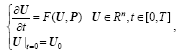 | , (1) |
where 


For a given prediction time T and a chosen norm, the perturbation 


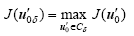
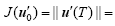
In this paper, 


The DE algorithm, a derivative-free and heuristic approach, was initially proposed by Storn and Price (1997). It belongs to the category of evolutionary algorithms. Many studies have applied evolutionary algorithms to study parameter estimates and the uncertainty of land surface models ( Duan et al., 1992; Kruger, 1993; Yapo et al., 1998; Zhang et al., 2000).
The method is a simple yet powerful population-based stochastic search technique. By mutation, crossover, and selection, it iterates continuously until the optimal value of the objective function over continuous space is obtained, or the number of iterations exceeds its preset maximum. Through extensive experiments ( Storn and Price, 1997), results have shown that the DE algorithm converges faster and has more certainty than many other acclaimed global optimization methods, e.g., Adaptive Simulated Annealing ( ASA; Ingber, 1993). In addition, it is robust and requires few control variables, and the reasonable choice of its control variables has been demonstrated in detail. Based on these characteristics, regardless of whether or not the objective function is differentiable, the DE algorithm can be used to tackle NOPs.
To date, the DE algorithm has only been applied to solve NOPs with box constraint conditions. However, in some studies, the CNOP is obtained for a NOP with a ball constraint condition. Therefore, in order to calculate CNOPs satisfying ball constraint conditions, the DE algorithm needs to be improved, in which a projection skill is first introduced. Projection skill has also been used in some traditional optimization algorithms aimed at solving optimization problems with ball constraint conditions, such as the SPG2 algorithm. Because of the randomized search strategy in the DE algorithm, the sampled member may lie outside the ball constraint. Thus, it is necessary to constrain this ŌĆ£outlierŌĆØ in a preset feasible region through projection skill. The projection skill used in the present study first involved the ŌĆ£outlierŌĆØ being normalized, and then multiplied by the radius of the ball constraint. Finally, the ŌĆ£outlierŌĆØ was projected onto the spherical surface, the border of the feasible region. Considering the CNOP is always located on the border of the feasible region, the DE algorithm could then quickly converge by applying this projection skill.
The SPG2 algorithm is a non-monotone projected gradient algorithm aimed at solving large-scale convex-con-strained optimization problems. It integrates the classical projected gradient method with the spectral gradient choice of steplength and a non-monotone line-search strategy. Further details can be found in Birgin et al. (2000). In calculating CNOPs, the adjoint-based method is used to obtain the derivatives of the cost function.
A simple model of the viscous BurgersŌĆś equation was employed, which describes the time evolution of the state variable uas follows:
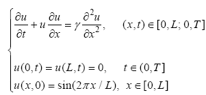 | , (2) |
where 
To explore the potential application of the DE algorithm (a derivative-free optimization approach) in calculating the CNOPs for NOPs with ball constraints, we designed a series of experiments that used the above mentioned numerical model and by perturbing the initial conditions. In order to verify the CNOPs obtained by the DE algorithm, the derivative-based optimization method (the SPG2 algorithm) was also applied to calculate the CNOPs for the same NOPs.
An initial perturbation 


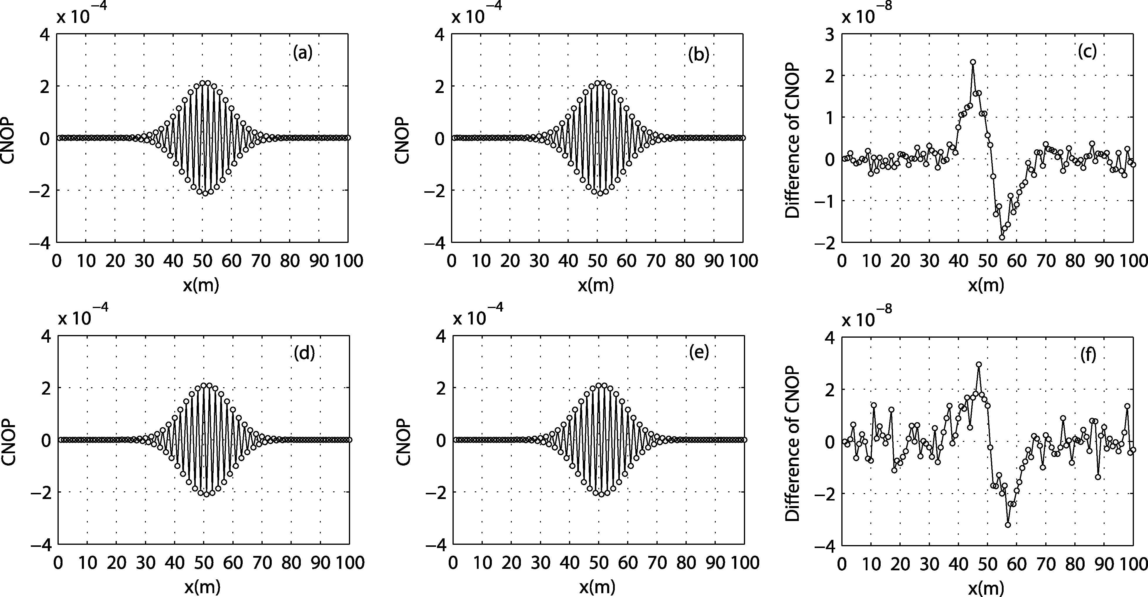
As demonstrated in Figs. 1a and 1b, the CNOPs calculated by the SPG2 and DE algorithms had almost identical spatial distributions, expect for small differences in magnitude (see Fig. 1c) when T= 30 s and n= 101. Although differences existed, the nonlinear time evolutions (in terms of their norm squares 
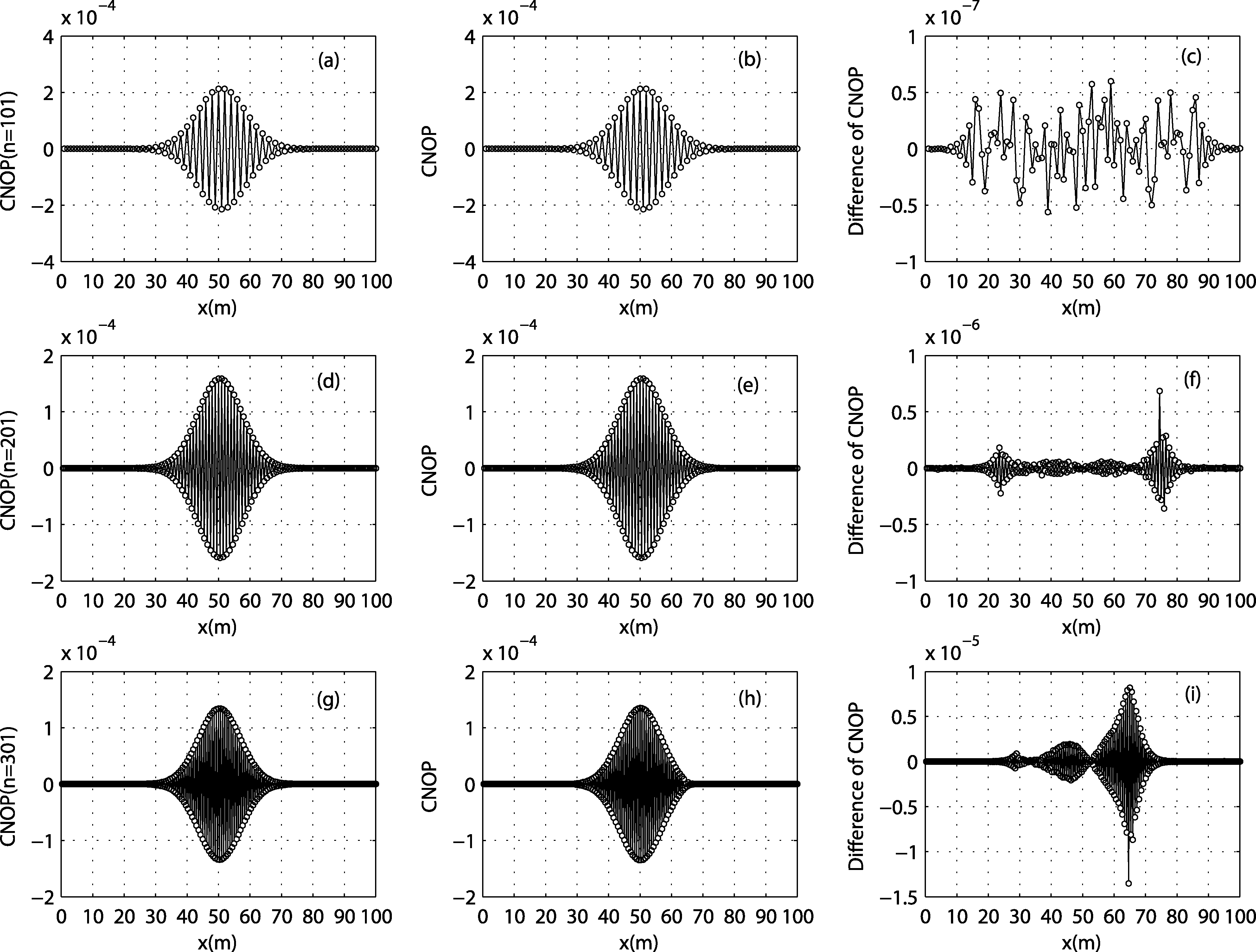 | Figure 1 Spatial distributions of CNOPs (m s-1) calculated by the (a, d, g) SPG2 algorithm and (b, e, h) DE algorithm, and the (c, f, i) CNOP differences (m s-1) (DE minus SPG2) when T= 30 s and n= 101, 201, 301, respectively (DE: the Differential Evolution algorithm; SPG2: the Spectral Projected Gradient algorithm). |
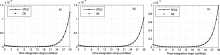
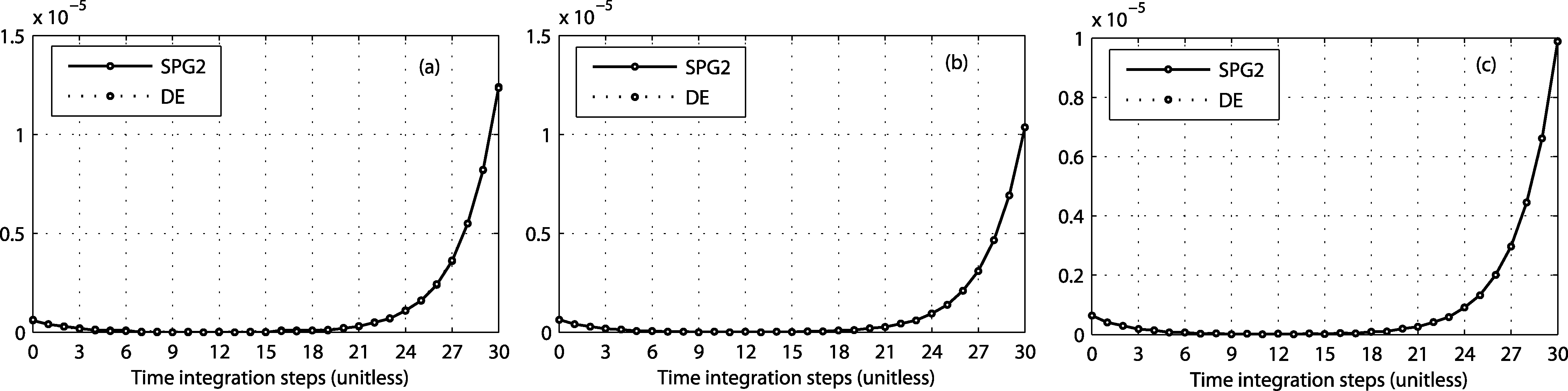 | Figure 2 Nonlinear evolutions of the CNOPs calculated by the SPG2 and DE algorithms when T= 30 s and n = (a) 101, (b) 201, and (c) 301. |
In order to study the dependence of the DE algorithmon the length of the prediction time in calculating CNOPs, we prolonged the prediction time T to 40 s and 50 s. Here, we only show the CNOPs obtained when n= 101 and T= 40 s, 50 s (see Fig. 3). Under other conditions (i.e., n= 201, 301), the results were similar. Little difference was found between the CNOPs obtained by the SPG2 and DE algorithms, and their nonlinear time evolutions were almost identical (data not shown). These findings illustrate that the DE algorithm could still be used to calculate CNOPs with increasing prediction time.
Table 1 summarizes the optimal values of the cost function in each experiment. At the same grid size and prediction time, the cost function values corresponding to the CNOPs calculated by the different algorithms were nearly the same. We also computed the correlation coefficients between the CNOPs obtained by the DE and SPG2 algorithms, all of which were greater than 0.99.
| Table 1 Summary of the optimal values of the cost function in the 18 numerical experiments. |
In conclusion, the derivative-free DE algorithm is able to calculate the CNOPs satisfying ball constraint conditions by being explanted to a projection skill. At the same spatial grid size and prediction time, the CNOPs obtained by the DE algorithm were nearly the same as those obtained by the SPG2 algorithm in terms of their spatial distributions and nonlinear evolutions. The DE algorithm is a good and reliable choice for obtaining CNOPs in complex models without available adjoint systems, or under the condition that the cost functions are non-differentiable.
 | Figure 3 Spatial distributions of CNOPs (m s-1) calculated by the (a, d) SPG2 algorithm and (b, e) DE algorithm, and the (c, f) CNOP differences (m s-1) (DE minus SPG2) when n= 101 and T= 40 s, 50 s, respectively. |
Many studies have indicated that the CNOP approach is a useful tool in atmospheric and oceanic studies. However, for complex numerical models without available adjoint systems, or under the condition that the cost functions are non-differentiable, it is difficult or impossible to obtain the CNOPs by using traditional gradient-based optimization methods.
To overcome this difficulty, we introduce the DE algorithm, a derivative-free method, together with a ball constraint condition and a projection skill to calculate the CNOPs by using a simple model of BurgersŌĆś equation. Through comparisons between the CNOPs obtained by the DE and SPG2 algorithms, we found that for the same NOP, the CNOP calculated by the DE algorithm was almost identical to that calculated by the SPG2 algorithm in terms of their spatial distributions and nonlinear time evolutions. Consequently, the DE algorithm has the potential to play an increasingly important role in calculating the CNOPs in future studies. The numerical results also imply that this algorithm can be applied to obtain the optimal values of optimization problems, especially for non-differentiable, nonlinear, and multimodal optimization problems.
However, the DE algorithm is far more computationally expensive than the SPG2 algorithm. Take the dimension of spatial grids n= 101 and prediction time T= 30 s as an example. During the optimization process, the SPG2 algorithm took less than 100 iterations. Meanwhile, after 100 iterations, the DE algorithm did not converge and the current optimal value of the cost function was just 1.0523E-05 (84.86% of the true maximum 1.2351E-05). At that moment, the current optimal initial perturbation calculated by the DE algorithm and the CNOP had similar spatial distributions except for differences in amplitudes and opposite phases, between which the correlation coefficient was -0.8660. In the subsequent iteration process, the current optimal perturbation obtained by the DE algorithm was converging to the CNOP slowly. In other words, many iterations (meaning more computation time) compensate for the lack of derivative information about the cost function during the search process of the DE algorithm. Nevertheless, with the rapid development of computers and the employment of parallel computing, the computation cost of the DE algorithm will be reduced greatly.
In this study, we only applied the DE algorithm to solve NOPs with dimensions of a magnitude of 100. Practically, the dimensions of NOPs in atmospheric and oceanic sciences always possess a magnitude of 103. In future, we will try to explore the application of the DE algorithm in these aspects.
Acknowledgments. The authors thank the anonymous reviewers for their suggestions to improve the manuscript. Funding was provided by grants from the LASG State Key Laboratory Special Fund and the National Natural Science Foundation of China (Grant Nos. 40905050, 40830955, and 41375111).
| 1 |
|
| 2 |
|
| 3 |
|
| 4 |
|
| 5 |
|
| 6 |
|
| 7 |
|
| 8 |
|
| 9 |
|
| 10 |
|
| 11 |
|
| 12 |
|
| 13 |
|
| 14 |
|
| 15 |
|
| 16 |
|
| 17 |
|
| 18 |
|
| 19 |
|
| 20 |
|
| 21 |
|
| 22 |
|
| 23 |
|
| 24 |
|
| 25 |
|
| 26 |
|
| 27 |
|
| 28 |
|
| 29 |
|
| 30 |
|
| 31 |
|
| 32 |
|
| 33 |
|
| 34 |
|