Bias Correction in Wind Direction Forecasting Using the Circular-Circular Regression Method
[XU Jing-Jing1, 2 , HU Fei2  , XIAO Zi-Niu
3, 4 , CHENG Xue-Ling2 ]
, XIAO Zi-Niu|
|


Wind direction forecasting plays an important role in wind power prediction and air pollution management. Weather quantities such as temperature, precipitation, and wind speed are linear variables in which traditional model output statistics and bias correction methods are applied. However, wind direction is an angular variable; therefore, such traditional methods are ineffective for its evaluation. This paper proposes an effective bias correction technique for wind direction forecasting of turbine height from numerical weather prediction models, which is based on a circular-circular regression approach. The technique is applied to a 24-h forecast of 65-m wind directions observed at Yangmeishan wind farm, Yunnan Province, China, which consistently yields improvements in forecast performance parameters such as smaller absolute mean error and stronger similarity in wind rose diagram pattern.
Wind direction forecasting has varied and important applications ranging from air pollution management to aircraft and ship routing and plays an important role in wind power prediction. Because of the terrain effects and other factors, such as wake effects caused by wind farm turbine arrangement, changes in wind direction cause large fluctuations in the output wind power in the entire wind farm ( Lange and Focken, 2006). However, the imperfections, approximations, and simplifications of numerical models lead to random and systematic errors that affect prediction accuracy. Therefore, post-processing bias correction of model output for wind direction is required. Because the impact of wind direction on output wind power is related to a given wind farm, the output wind power can generally be calculated by the power curve of the given wind farm, in which wind speed and wind direction are the most important impact factors ( Burton et al., 2001).
However, wind direction is an angular variable that has values on the circle; other weather quantities such as temperature, precipitation, and wind speed are linear variables that have values on the real line. Therefore, traditional post-processing techniques for forecasting from numerical weather prediction models tend to become ineffective for wind direction. Engel and Ebert (2007) observed that bias correction was not beneficial for wind direction forecasting. For wind, the traditional approach develops separate model output statistics (MOS) equations ( Glahn and Lowry, 1972) for the zonal and meridional components from which single-valued forecasts of wind speed and wind direction are derived. However, because this approach does not consider the dependencies between wind speed and wind direction, it can lead to biases ( Carter, 1975; Glahn and Unger, 1986). Probabilistic forecasting for angular quantities has been discussed by Grimit et al. (2006) and Bhattacharya and Sengupta (2009).
Bao and Gnetting (2010) adopted a different approach to predicting wind direction by proposing the use of a circular-circular regression technique. Models employing this technique have been discussed by Fisher and Lee (1992) and Fisher (1993). Earlier works on directional statistics in which the Mobius transformation appeared include that by McCullagh (1996). Downs and Mardia (2002) proposed a regression model in which the regression curve is expressed as a form of the Mobius transformation, with application to data on circadian biological rhythms and wind direction. Minh and Farnum (2003) induced probabilistic models on the circle using a bilinear transformation, which is related to the Mobius transformation. Kato et al. (2008) obtained properties of the regression, including estimation and testing procedures, and the proposed methods are applied to marine biology and wind direction data.
The purpose of this paper is to apply the circular- circular regression bias correction approach to wind direction forecasting of wind turbine height for wind power prediction. The remainder of the paper is organized as follows. In section 2, we describe our approach to bias correction in detail. The model and set-up of experiments are introduced in section 3. Section 4 provides a one-year case study on a 24-h forecast of wind direction in the Yangmeishan wind farm in 2012. Conlcusions are given in section 5.
The von Mises distribution, which is unimodal circular distribution, is a natural baseline for modeling angular data such as wind direction and may be viewed as a circular analog of Gaussian distribution ( Fisher, 1993). In particular, an angular variable is believed to have a von Mises distribution with mean direction μ and concentration parameter κ, if it has density
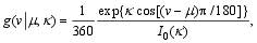 | (1) |
on the circle, where v denotes the observed wind direction, and I0 is a modified Bessel function of the first kind and order zero. As the concentration parameter κ approaches to zero, the von Mises distribution becomes a uniform distribution on the circle. If the distribution of the angular variable on a circle has the trend of concentration in a direction and is not uniformly distributed by the test it is known as a unimodal circular distribution. On the contrary, if the angular variable is uniformly distributed on the circle and has no obvious concentration tendency, the mean angle does not exist.
Mobius transformation is well known as a mapping that carries the complex plane onto itself. With some restrictions on the parameters, Mobius transformation maps the unit circle onto itself or the unit circle onto the real line. Because the Mobius transformation is diffeomorphic, it can be regarded as equivalent transformation. Therefore, the circular-circular regression based on Mobius transformation is equivalent to the linear regression for linear varibles.
Bao and Gnetting (2010) proposed a nonlinear regression equation of the form
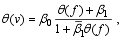 | (2) |
where f denotes the predicted and observed wind direction, and θ( f ) and θ( v) denote the associated points on the unit circle in the complex plane, as described below:
 | (3) |
where β0 is a complex number with modulus | β0|=1 and β1 is any complex number. The bar denotes complex conjugation. The mapping from θ( f ) to θ( v) is a Mobius transformation in the complex plane, which is one-to-one, and maps the unit circle onto itself. The regression parameters β0 and β1 must be estimated from training data. Whereas β0 is a rotation parameter, β1 indicates pulling a direction toward a fixed angle that is, the point β1/| β1| on the unit circle ( Kato et al., 2008).
In our circular-circular regression approach to bias correction for wind direction, we estimate the Mobius transformation Eq. (2) from training data by numerically minimizing the sum of the circular distances between the fitted bias-corrected forecasts and the respective verifying directions as a function of the regression parameters ( Lund, 1999). The angular distance or circular absolute error
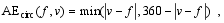 | (4) |
between two directions 0≤ f, v<360 is a non-negative quantity with a maximum of 180°. Because the training data comprises the pairs of predicted and observed directions, the mean circular absolute error is:
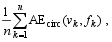
In this paper, we use degrees to describe predicted and observed wind direction, with 0°, 90°, 180°, and 270° denoting northerly, easterly, southerly, and westerly wind, respectively.
The bias correction method described in section 2 is applied to a 24-h forecast determined by the Weather Research and Forecasting (WRF) model based on 65-m (wind turbine height) wind directions measured in 10-min increments, which was issued at 1800 UTC everyday ( Skamarock et al., 2008). The WRF model is applied over southwestern China with three nested domains centered over Yunnan Province with 27-km, 9-km, and 3-km horizontal grid increments and 37 vertical levels, 12 of which are located in the lowest 1 km. The parameterizations chosen for these experiments include the Purdue Lin microphysics scheme ( Lin et al., 1983), the Mellor-Yamada- Janjic planetary boundary layer (PBL) scheme ( Mellor and Yamada, 1982), the Monin-Obukhov scheme ( Monin and Obukhov, 1954) for the surface layer, the Kain-Fritsch scheme ( Kain, 2004) for the convective processes (only in the two coarser domains), and the Noah land surface model ( Chen and Dudhia, 2001) or the land surface scheme.
The bias correction method described above was tested with observation for a period of approximately one year, from 03 April 2011 to 02 May 2012, from one mast situated at the Yangmeishan wind farm, Yunnan Province, China. The observation station, at 25°06′N, 103°49′E, and altitude 2210 m, is located within the finest inner domain. Model 65-m wind component forecasts at the four grid- box centers surrounding the station were bilinearly interpolated to the observation location. The station is located in typical terrain that includes Yangmeishan Mountain with high elevation and complex topography.
For pre-processing of the bias correction, we first obtained 1-h average wind velocities, which were in-turn obtained by composing six time wind vectors of 10 min. Our verification results included forecast-observation cases only when the verifying wind speed was at least 3 m s-1 because wind direction observations are unreliable at lower wind speeds. In view of this constraint, forecast- observation cases at the given station were available for 341 days. The bias correction used the seven-day observed wind direction during the sliding training period.
In section 2, we proposed a method for bias correction of angular variables, that is, circular-circular regression, which employs a nonlinear regression approach specific for circular data. In this section, we applied the bias correction method for verification.
We individually fit the bias correction scheme for each training period to examine the sensitivity of the length of the sliding training period. Table 1 shows the mean circular absolute error for sliding training periods ranging from 7 to 49 days averaged over 292 days; 49 days were removed as the initial training period. Because weather patterns change over time, there is an advantage in using a short training period to adapt to such changes. However, longer training periods result in lower estimation variance. The training sets were constrained to cases at the station and the periods were extended in the case of missing data. For example, the seven-day training period always used the 168 most recent available forecast cases.
| Table 1 Mean circular absolute error (units: °) for raw and bias-corrected 24-h forecast of 65-m wind direction at Yangmeishan wind farm, Yunnan Province, China. The results are averaged over a one-year period for sliding training periods of lengths 7, 14, 21, 28, 35, 42, and 49 days. |
The circular absolute error of the raw forecast was 25.4°. For a seven-day training period, the raw forecast outperformed the circular-circular regression. However, as the training period increased, circular-circular regression became the method of choice. This result was expected because more complex statistical methods require larger training sets to avoid overfitting. Overall, circular-circular regression with training periods of 14 days or more performed better. When the training period exceeded 42 days, the bias correction effects became steady. On average, the circular absolute error was reduced by 2° or 3° over that of the raw forecast.
Therefore, in subsequent results, we analyzed the cases in which the regression parameters in Eq. (2) were fit on a 42-day sliding training period.
First, we selected a typical day to obtain an intuitive image. The specific example is a forecast of 65-m wind direction at Yangmeishan wind farm, Yunnan Province, China, issued on 26 November 2011. The circular-circular regression scheme for bias correction was estimated on a 42-day training period immediately preceding the initialization date.
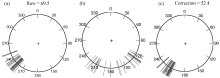
Figure 1 illustrates the raw and bias-corrected forecast at Yangmeishan wind farm along with the observation for a reference forecast. The reference forecast used the 42-day observed wind direction during the sliding training period. The blue lines and graphs represent the forecast distributions. The illustration shows that the wind direction of observation is uniformly distributed between 120° and 210°, whereas the raw output density is centered at 230°, and the bias correction technique results in counterclockwise rotations by approximately 20°, and thus, gets the contraction of 210°. The circular absolute error of the day was considerably smaller for the bias-corrected forecast distribution, at 52.4°, than that for the raw forecast. Moreover, the bias correction technique reduced the circular absolute error of 17.1°.
 | Figure 1 Circular diagrams of forecast distributions for wind direction at Yangmeishan wind farm, Yunnan Province, China, measured on 26 November 2011: (a) raw, (b) observation, and (c) bias-corrected. The black lines and graphs represent the forecast distributions. The circular absolute error of the day is shown in degrees. |
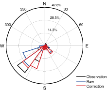
The wind rose diagram is a histogram of the circular variable and can visually represent the general distribution of wind direction. Figure 2 shows the wind rose diagram of forecast distributions for wind direction at Yangmeishan wind farm. The annual observed winds are mostly southwest and southerly. The model simulated the basic patterns of annual wind direction; however, the simulation was more westerly. The pattern of bias-corrected wind direction showed stronger similarity to the observation, and the primary improvement was located between west and south, which is the main distribution area of wind direction. The improvement of two 18° sector regions of 198-216°E and 234-252°E was particularly obvious, and the bias-corrected wind direction became much closer to observation.
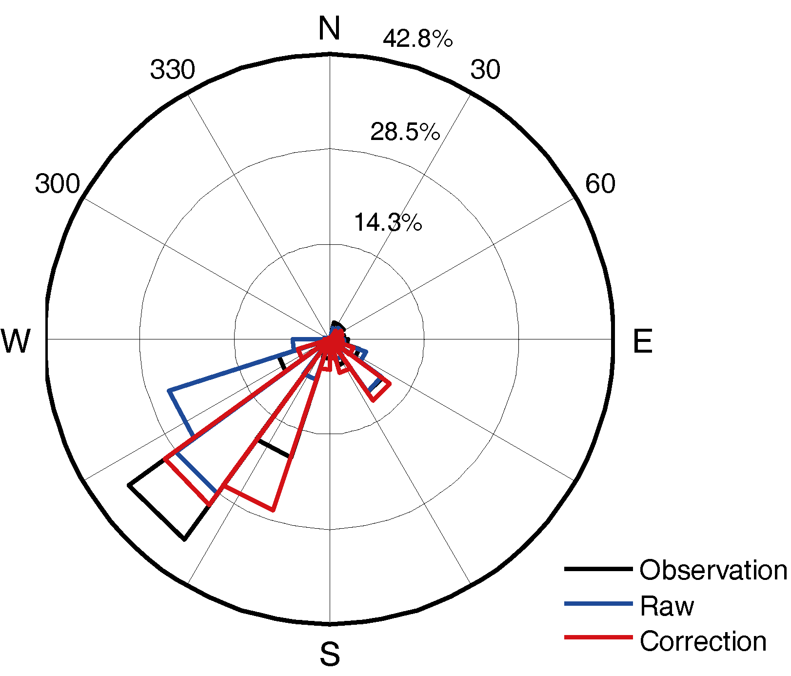 | Figure 2 Wind rose diagram of forecast distributions for wind direction at Yangmeishan wind farm, Yunnan Province, China. Black lines represent the forecast distributions of observation, blue lines represent raw output, and red lines represent bias-corrected results. |
As shown in Table 2, the following five metrics were computed to evaluate the performance of the bias correction method:
a) The mean direction 
b) The length of the mean resultant vector 

c) The circular variance defined as S= 1- R; the circular variance S lies in the interval [0, 1].
d) The angular deviation defined as 

e) The correlation coefficient ρcc between two directional random variables α and β by
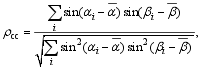 | (6) |
where 
As indicated in Table 2, the mean direction of observation was 198.7°, which is located southwest, and the mean of raw output was 211.9°, which is 13.2° more westerly than the observation. Otherwise, the mean direction of bias correction was 196.1°, which shows a decrease of 15.8° over the raw output and is much closer to the observation. The correlation coefficient is also an important quantity. The circular-circular correlation coefficient of observation and raw output was 0.70, which suggests a strong correlation, and the correlation coefficient of observation and bias correction was 0.71, which shows further improvements. The circular variance and circular standard deviation both describe the contraction extent of the circular variable. The circular variance of observation was 0.37 and that of raw was 0.41, indicating a smaller contraction extent for the observation. The circular variance of bias correction was 0.30, which is significantly smaller than that of observation. We can derive a similar conclusion for the circular standard deviation. Because of the characteristics of the bias correction method, the raw output of the three quantities, including the resultant vector length, outperforms the bias correction.
| Table 2 Evaluation metrics of the bias correction method, including mean direction, resultant vector length, circular variance, circular standard deviation, and circular-circular correlation coefficient, which denotes the circular-circular correlation coefficient of observation and raw output and the correlation coefficient of observation and bias correction, respectively. |
In this paper, the bias correction method was applied to 24-h wind direction forecast at a 65-m height at the Yangmeishan wind farm. We have demonstrated the method for performing bias correction for wind direction, which is an angular variable. For this method, we used the circular-circular regression approach, which employs a Mobius transformation to regress the verifying wind direction on the model wind direction. A possible extension is the regression model of Lund (1999), which allows for additional linear predictor variables such as the model wind speed. To estimate the regression parameters, we used a minimum circular absolute error criterion. On the basis of these experiments, the bias correction method was determined to be effective, yielding consistent improvements in forecast performance.
We first performed the sensitivity test of the length of the sliding training period. For a seven-day training period, the raw outperformed the circular-circular regression. However, as the training period increased, circular-circular regression was preferred. Overall, circular-circular regression with training periods of 14 days or more performed better. When the training period exceeded 42 days, the bias correction effects became steady. On average, the circular absolute error was reduced by 2° or 3°, compared with that of the raw forecast. The annual observed winds were mostly southwest and southerly, whereas the simulation was more westerly. The pattern of bias-corrected wind direction showed stronger similarity to the observation. The primary improvement was located between west and south, which was the main distribution area of wind direction. Moreover, the bias correction outperformed the raw output of the mean direction and the circular-circular correlation coefficient.
| 1 |
|
| 2 |
|
| 3 |
|
| 4 |
|
| 5 |
|
| 6 |
|
| 7 |
|
| 8 |
|
| 9 |
|
| 10 |
|
| 11 |
|
| 12 |
|
| 13 |
|
| 14 |
|
| 15 |
|
| 16 |
|
| 17 |
|
| 18 |
|
| 19 |
|
| 20 |
|
| 21 |
|
| 22 |
|
| 23 |
|