
Assessment of Historical Climate Trends of Surface Air Temperature in CMIP5 Models
[FENG Xiao-Li1 , ZHI Hai1 , LIN Peng-Fei2  , LIU Hai-Long
2 ]
, LIU Hai-Long|
|


This study assesses the historical climate trends of surface air temperature (SAT), their spatial distributions, and the hindcast skills for SAT during 1901- 2000 from 24 Coupled Model Intercomparison Project Phase 5 (CMIP5) models. For the global averaged SAT, most of the models (17/24) effectively captured the increasing trends (0.64°C/century for the ensemble mean) as the observed values (~ 0.6°C/century) during the period of 1901-2000, particularly during a rapid warming period of 1970-2000 with the small model spread. In addition, most of the models (22/24) showed high hindcast skills (the correlation coefficient,
The global averaged surface air temperature (SAT) has increased by 0.74°C during 1906-2005 according to the Fourth Assessment Report of the Intergovernmental Panel on Climate Change ( IPCC, 2007). Warming is not continuous; it has occurred principally during two periods from 1920 to 1945 and from 1975 to the present ( Sakaguchi et al., 2012). The variable warming spatial pattern, which has gained increasing acceptance, displays various influences on local weather and climate change ( Jiang et al., 2005; Smith et al., 2010; Sun et al., 2010).
Coupled models are often used to detect natural and anthropogenic components of observed trends by testing alternative scenarios driven with natural forcing or that combined with anthropogenic forcing ( Jones et al., 2013; Knutson et al., 2013). However, many uncertainties remain in model simulations, which limit the precision and accuracy of their results. Simulation uncertainties result mainly from model biases such as deficiencies in model resolution or its physical processes. To precisely assess the warming, sufficient ensemble members from various complex climate models are needed to lower the uncertainty from a simple climate model and few members simulated by few complex climate models ( Gillett et al., 2002; Jiang et al., 2012). For the regional scale, many approaches and schemes based on dynamical models, statistical methods, and their combinations have been developed to improve simulation skills ( Gao et al., 2001; Zhang et al., 2008).
Several studies have estimated 20th century temperature trends or simulation skill at global and regional scales by using selected Coupled Model Intercomparison Project Phase 3 (CMIP3) models ( Zhou and Yu, 2006; Sakaguchi et al., 2012). At sub-continental or larger scales, SAT trends can be reproduced by most CMIP3 models. Such warming trends and skills in CMIP5 models require further study.
Researchers have attempted to explore the factors that control changes in surface temperature by analyzing observational data based on the Earth’s global energy budget ( Andrews et al., 2009; Murphy et al., 2009). In fact, the conclusions drawn from such observations often show conflicting results ( Zhang et al., 1995; Qu et al., 1998). Thus, it is necessary to demonstrate whether SAT trends correlate with heat fluxes at the top of the atmosphere (TOA) and at the Earth’s surface.
Our objectives of the present study are to perform an assessment of historical SAT trends and their hindcast skills in selected CMIP5 models and to explore the possible causes of such SAT trends. A description of CMIP5 models and reanalysis data used for comparison is given in section 2. Section 3 presents the results and possible causes of these trends, and a summary and discussion is presented in section 4.
In this study, we used 24 CMIP5 models and their outputs ( Taylor et al., 2012) from historical runs. SAT and each component of heat fluxes at the TOA and at the surface in these models are available on the CMIP website (http://www-pcmdi.llnl.gov/projects/cmip/). Table 1 shows CMIP5 model information including the assigned model number of the model name, affiliated country, ensemble members, and horizontal resolution in the atmospheric component. SATs from the National Aeronautics and Space Administration Goddard Institute for Space Studies Surface Temperature Analysis (GISTEMP) ( Hansen et al., 1999) and the Met Office Hadley Centre and Climatic Research Unit Latest Version (HadCRUT4) ( Morice et al., 2012) served as observations and were used for comparison in this study. In addition, we used related variables from the 20th Century Reanalysis Version 2 provided by the National Oceanic and Atmospheric Administration Cooperative Institute for Research in Environmental Sciences (20CRv2) ( Compo et al., 2011), including longwave radiation, shortwave radiation, latent heat flux, and sensible heat flux at the surface.
| Table 1 CMIP5 models used in this paper are listed with countries, ensemble members, and the horizontal resolutions in the atmospheric component. Each model is labeled with a code number. |
Each modeling center submitted multiple ensembles for historical simulation. We used the ensemble mean of several members for each model (Table 1). For ease in comparison and evaluation, we remapped SAT to a 1° × 1° gird evenly by using bilinear interpolation. The climatologically monthly mean values of 1971-2000 were subtracted from the monthly mean SATs, and a 10-year running mean was applied to remove interannual signals such as El Niño Southern Oscillation (ENSO). Linear least squares fit was used to compute linear trends of the 10-year running mean monthly SAT anomaly. Hindcast skills were estimated by determining the Pearson product-moment correlation coefficients ( R) between observation and models. The root mean square deviation (RMSD) relative to the ensemble mean was computed to quantify intermodel spread.
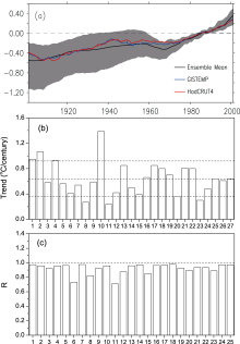
The time series of global averaged SAT anomalies from observations and simulations displayed obvious warming signals of the 20th century (Fig. 1a). The ensemble mean captured the increase in SAT of approximately 0.3°C from 1910 to 1940 and a slight cooling trend from 1940 to 1970 as observed values but had a large intermodel spread. The models captured a rapid warming of > 0.5°C from 1970 to 2000 more effectively than slow warming from 1910 to 1940 and from 1940 to 1970 due to the small model spread; these results are similar to those of CMIP3 1880-1899 climate simulations with the exception of the model spread size ( Zhou and Yu, 2006).
Quantitatively, during 1901-2000, the SAT trends estimated from GISTEMP and HadCRUT4 were 0.61 °C/century and 0.62°C/century, respectively (Fig. 1b). The simulated trends showed considerable spread of 0.2-1.4°C/century among the 24 CMIP5 models, although their ensemble mean value of 0.64°C/century was close to that of the observed values (Fig. 1b). Eleven (thirteen) models overestimated (underestimated) the warming. For model 10, the warming trend in SAT was the largest, whereas that in model 11 was the smallest. Trends in seven models including 1, 2, 4, 8, 10, 11, and 23 exceeded 1 RMSD relative to the ensemble mean value. Temporal changes in SAT between GISTEMP and HadCRUT4 were highly consistent (Fig. 1a); thus, we selected one of the observation datasets, GISTEMP, to calculate the R between each model and observation during 1901-2000. As expected, the R exceeded 0.8 in 22 of the 24 models (Fig. 1c). This result indicates that most of the models had relatively high hindcast skills for the global mean SAT, which is higher than those of R > 0.5 in most of the CMIP3 models ( Zhou and Yu, 2006).
 | Figure 1 (a) Time series of globally averaged 10-year running mean surface air temperature (SAT) anomalies (°C, 1901-2000) determined by models and observations (Goddard Institute for Space Studies Surface Temperature Analysis (GISTEMP) and the Met Office Hadley Centre and Climatic Research Unit Latest Version (HadCRUT4)), (b) their linear trends (°C/century), and (c) correlation coefficients between each model and GISTEMP. The gray shaded areas in (a) represent the zones between the maximum and minimum values from the 24 models. The x-axes in (b) and (c) are labeled with the 24 model numbers shown in Table 1 and their ensemble mean value, shown in the 25th column. The 26th and 27th columns in (b) represent observed trends from GISTEMP and HadCRUT4, respectively. The black dashed lines in (b) indicate the locations of the ensemble mean trend and ensemble mean trend ± 1 RMSD. |
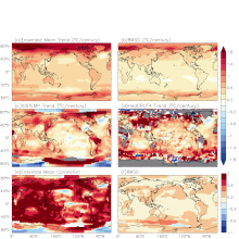
To test whether the trends showed spatial differences, the distribution of the ensemble mean SAT trends was determined (Fig. 2a). The obvious warming on the land indicated in the observation (Figs. 2c and 2d) was essentially captured in the ensemble mean of the models (Fig. 2a); however, the warming patterns differed. In the observations, the most obvious warming was located mainly on the Eurasian continent between 40°N and 70°N, although the magnitudes of the trends differed between GISTEMP and HadCRUT4. The most obvious warming determined by most of models, > 1.4°C/century, was situated north of 55°N. In the North Atlantic between 40°N and 60°N, the ensemble mean captured the same cooling as that in observations but with a large model spread (Figs. 2a and 2b).
 | Figure 2 (a) Ensemble mean SAT linear trends (°C/century) and (b) the root mean square deviation (RMSD) of SAT linear trends from 24 models during 1901-2000, SAT linear trends from (c) GISTEMP and (d) HadCRUT4, (e) ensemble mean correlation coefficients between simulated and observed SAT time series, and (f) RMSD of correlation coefficients from the models. |
The simulated historical warming on the land was larger than that in the ocean between 40°S and 40°N in most models (Figs. 2a and 2b). The land warming was underestimated as compared with that determined by GISTEMP and HadCRUT4. Meanwhile, obvious warming along several oceanic boundaries, such as those along the Kuroshio extension and the East China Sea, and the slight cooling in some regions such as the central equatorial Pacific and the southwest Indian Ocean, were not captured by most of the models.
In the middle-to-high latitudes of the Southern Hemisphere, the warming trends were less than 1.4°C/century. The most obvious simulated trends were located in the Southern Ocean near land, particularly between the Pacific and Atlantic sectors. Moreover, large model spread was apparent in the most obvious warming regions, which indicates that the trends differed among models. In fact, observations contain large amounts of missing data, and the conclusions drawn from such observations often show conflicting results ( Thorne et al., 2011). Limited data coverage precludes an assessment of SAT trends over the Arctic Ocean, Antarctica, and the Southern Ocean south of 40°S, which are represented in Fig. 2d as gray areas on the HadCRUT4 map.
The spatial distribution of ensemble mean correlation coefficients between simulated and GISTEMP SAT are presented in Fig. 2e. Relatively high hindcast skills of R > 0.6 were shown in most regions excluding Antarctica, some parts of the Pacific Ocean, the North Atlantic Ocean between 40°N and 60°N, the Southwest Indian Ocean, and the Arctic Ocean. The intermodel hindcast skills ranged from 0.0 to 0.3 with large uncertainty in the Southern Ocean between the Indian and Pacific sectors (Fig. 2f). These results indicate that the present coupled models have some capabilities for simulating the broad-scale features of SAT trends, which closely follows the effective simulation results of the CMIP3 models for showing the probability distribution of trends during the 20th century ( Easterling and Wehner, 2009).
To examine the relationship between SAT tendency and heat fluxes at the TOA and at the surface on > 10-year time scales, their correlations were calculated after the 10-year running mean was applied. The significant positive correlations indicate that SAT trends can be attributed to the changes in the net TOA radiation flux and in the net surface heat flux (Figs. 3a and 3e). For the climate system at the TOA, the gained heat drove the positive SAT trend, and the increase in net surface heat flux caused an increase in SATs.
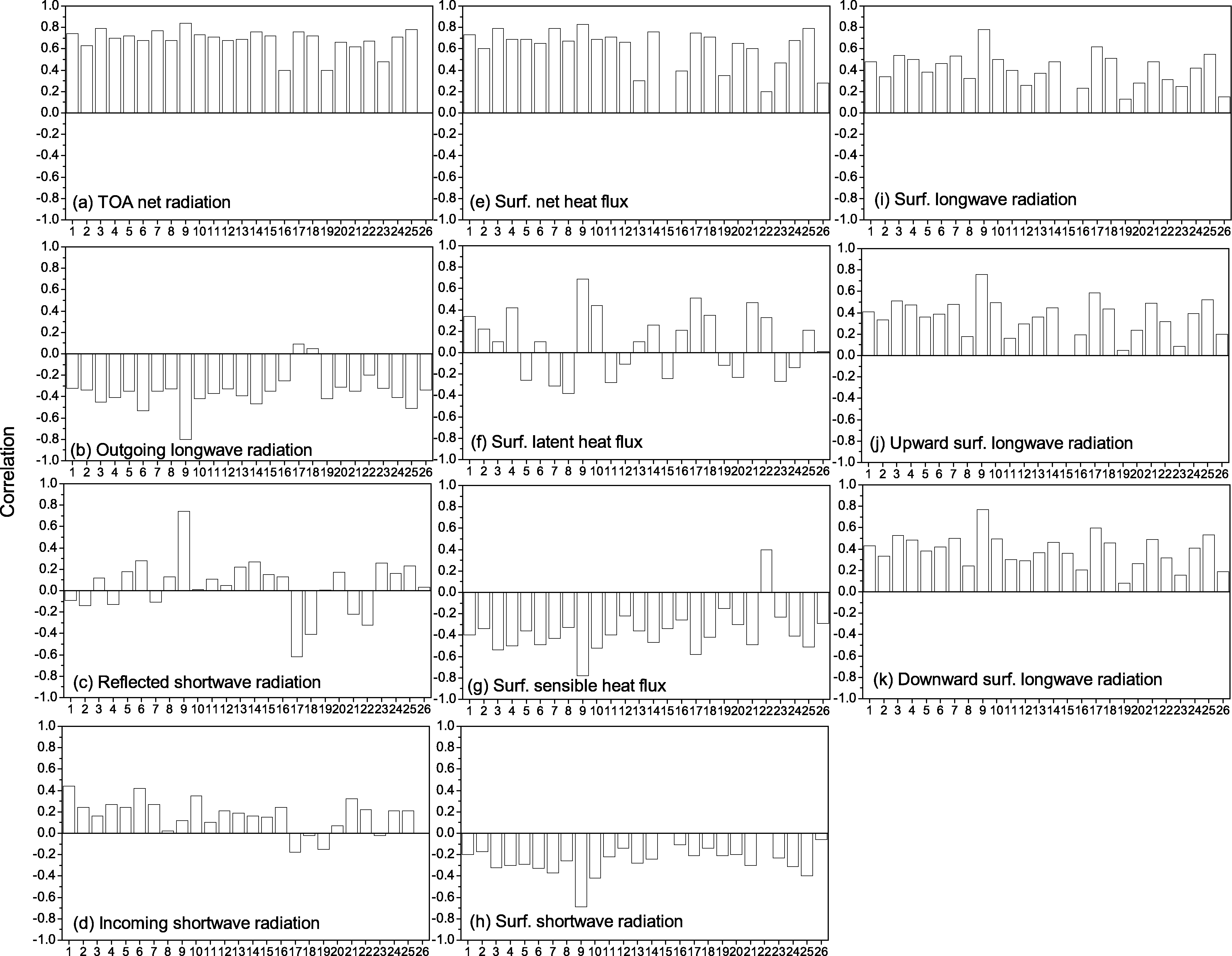 | Figure 3 Correlation coefficients between SAT tendencies and each component of heat fluxes including (a) net TOA radiation flux, (b) OLR at the TOA, (c) RSW at the TOA, (d) ISR at the TOA, (e) net surface heat flux, (f) surface LH flux, (g) surface SH flux, (h) surface SW, (i) surface LW, (j) upward surface LW, and (k) downward surface LW. The SAT tendencies were determined after the 10-year running mean SAT globally averaged anomalies were applied during 1901-2000. The x-axes are labeled with the 24 model numbers shown in Table 1. The 25th and 26th columns represent the correlations from the ensemble mean and the reanalysis, respectively. |
The TOA radiation fluxes include outgoing longwave radiation (OLR, positive upward), reflected shortwave radiation (RSW, positive upward), and incoming shortwave radiation (ISR, positive downward). The relationships between these three radiation flux components at the TOA with SAT tendency are given in Figs. 3b, 3c, and 3d. The correlations between SAT tendency and OLR were significantly negative in 22 of the 24 models, which indicate that a decrease in OLR can result in an increase in SAT. The positive (negative) correlations between SAT tendency and RSW existed in sixteen (eight) models. The obvious negative correlations in the models 17, 18, 21, and 22 caused the increase in SAT. ISR showed a positive correlation with SAT tendency, which indicates that ISR can lead to an increase in SAT. Thus, at the TOA, the increase in SAT resulted mainly from the increase in ISR and decrease in OLR in most of the models, and the RSW curtailed the increase in SAT in two-thirds of the models.
In Figs. 3e-k, relationships between every heat flux component at the surface and SAT tendency are given to examine their contributions to the warming. The surface heat fluxes include latent heat flux (LH, positive upward), sensible heat flux (SH, positive upward), net longwave radiation (LW, downward minus upward), and net shortwave radiation (SW, downward minus upward). The relationships were consistent between LW, SW, and SAT tendency in the models and reanalysis data (Figs. 3f and 3h). The correlation between SH and SAT tendency was consistently negative in the observation and in 22 models, whereas the relationship between LH and SAT tendency showed large inconsistencies, for which many findings have been challenged ( Zhang et al., 1995; Qu et al., 1998; Andrews et al., 2009). The consistently negative correlations between SAT tendency and SW indicate that SW curtailed the increase in SAT. SH led to the increase in SAT due to the consistently negative correlations. The decrease in SH may be attributed to the decrease in temperature difference between the atmosphere air temperature and surface temperature or a decrease in surface wind speed. This relationship indicates that LW can result in an increase in SAT. Although the upward LW showed a positive correlation with SAT tendency, upward LW did not induce an increase in SAT. The positive correlation between downward LW and SAT tendency indicates that the increase in SAT resulted from the increase in downward LW, which was due to an increase in greenhouse gases. This process is a classic interpretation of global warming because of the large upward LW and large downward LW. Uncertainty existed in correlations between SAT tendency and LH among models; 14 models showed positive correlation and 10 models showed negative correlation. Thus, the net surface heat flux was affected mainly by SH and LW (LW effect is due to greenhouse gases effect). Most of the models showed a somewhat higher correlation than that of the reanalysis data, which indicates that the models are effective tools for studying SAT tendency.
In this study, we used 24 CMIP5 models to estimate the historical climate trends of SAT, their distributions, and hindcast skills for SAT during 1901-2000. The possible causes of SAT trends were explored by examining the relationships between SAT tendency and heat fluxes at the TOA and at the surface.
The simulated trends of global averaged SAT during 1901-2000 were comparable to the observed trends estimated from GISTEMP and HadCRUT4. The models were better able to consistently capture the rapid warming between 1970 and 2000 than the slow warming between 1901 and 1970. Most models (22/24) showed high hindcast skills for the global averaged SAT with R > 0.8.
The simulations and observations displayed similar spatial patterns such that the warming at the middle-to- high latitudes in the Northern Hemisphere was greater than that in the Southern Hemisphere, and warming on land was greater than that in the ocean between 40°S and 40°N. The simulations underestimated the warming along some ocean boundaries and on land and overestimated the warming in the Arctic Ocean. In addition, the large model spread in the most obvious warming regions implies large differences among models.
Relatively high hindcast skills of R > 0.6 were shown in most regions except for the Arctic Ocean and the cooling regions shown in the observation. The present coupled models have the capability of simulating the broad-scale features of SAT trends except in the Southern Ocean between the Indian and Pacific sectors due to the small model skill spread.
The relationships between heat fluxes at the TOA and the surface and SAT tendency indicate that net heat fluxes can contribute to the warming. At the TOA, the OLR and ISR showed positive effects of the warming in most models. At the surface, the LW and SH led to the SAT warming in most models. The downward LW effectively contributed to the warming, whereas SW slightly curtailed the increase in SAT. Moreover, the relationship between SAT tendency and LH differed among models.
| 1 |
|
| 2 |
|
| 3 |
|
| 4 |
|
| 5 |
|
| 6 |
|
| 7 |
|
| 8 |
|
| 9 |
|
| 10 |
|
| 11 |
|
| 12 |
|
| 13 |
|
| 14 |
|
| 15 |
|
| 16 |
|
| 17 |
|
| 18 |
|
| 19 |
|
| 20 |
|
| 21 |
|
| 22 |
|