Determining the climate trend is an important step in statistics and numerous scientific analyses, and is key for estimations of global warming. Most studies addressing possible climate trends in climate datasets assume a priori that the trends are linear and consequently use least squares linear fitting (LSLF) to extract the trend (e.g., Born, 1996; Dai et al., 1997; Norris, 2005; Stocker et al., 2013). Linear trend analysis can estimate the quantitative trend in a simple way. However, estimating the climate trend using the linear approach is not physically realistic and can lead to uncertainty because the temporal behavior is complex in a changing climate (e.g., Wu et al., 2011; Qin et al., 2012). The ensemble empirical mode decomposition (EEMD) approach (Wu and Huang, 2009) can extract the temporally changing nonlinear trends (Franzke, 2009, 2010, 2012; Wu et al., 2011) from a changing complex climatic time series.

Coupled models are often used to detect/attribute historical observed trends by testing alternative scenarios driven by different forcings (e.g., natural, anthropogenic) (Jones et al., 2013; Knutson et al., 2013). The first step is to access and estimate the historical trends precisely from coupled climate models. However, due to biases and internal variability from different models, using just one model can bring relative large uncertainty. To combat this problem, multiple models are instead often used. The Coupled Model Intercomparison Project Phase 5 (CMIP5) has provided simulation results from multiple models. Evaluating the CMIP5 simulations using EEMD can help us understand the simulation abilities.

The aims of this study are to estimate and assess the historical climate trends from multiple CMIP5 models and observations using the EEMD and LSLF methods, and compare the surface air temperature (SAT) trends in different periods. The temporally changing nonlinear and linear trends are presented during the slow warming period and the rapid warming period. The possible differences in the trend lines and their causes in the slow and rapid warming periods according to the two approaches are explored. A brief description of the data and methods is given in section 2, follows by the results in section 3, and a brief summary in section 4.

We select the first ensemble member (i.e., “ r1i1p1” ) in the historical runs forced by greenhouse gases, sulfate aerosols, and volcanic and solar activity during the period of 1850 (or 1860) to 2005 from 27 CMIP5 models (Taylor et al., 2012). Table 1 shows the details of the CMIP5 models, including the assigned model number for each model name, the modeling center, the affiliated country, and the reference (or link). SATs simulated by the models are compared with observed SATs from the the National Aeronautics and Space Administration Goddard Institute for Space Studies Surface Temperature Analysis (GISTEMP) (Hansen et al., 1999) and the Met Office Hadley Centre and Climatic Research Unit latest version (HadCRUT4) (Morice et al., 2012) datasets.

Table 1

Table 1

Table 1 Details of the Coupled Model Intercomparison Project Phase 5 (CMIP5) models used in this paper, including their modeling centers, countries (organizations), and references (or links) for the atmospheric component. Each model is labeled with a code number. Model No. Model name Modeling center Country/organization Reference or link 1 BCC-CSM1.1 BCC China Xin et al. (2013) 2 BNU-ESM GCESS China http://esg.bnu.edu.cn/BNU_ESM_webs/html_webs/html 3 CanESM2 CCCMA Canada Chylek et al. (2011) 4 CCSM4 NCAR USA Gent et al. (2011) 5 CESM1-CAM5 NSF-DOE-NCAR USA Meehl et al. (2013) 6 CMCC-CM CMCC Italy http://www.cmcc.it/website/models 7 CNRM-CM5 CNRM-CERFACS France Voldoire et al. (2013) 8 CSIRO-Mk3-6-0 CSIRO-QCCCE Australia Rotstayn et al. (2010) 9 EC-EARTH EC-EARTH Europe Hazeleger et al. (2012) 10 FGOALS-g2 LASG-CESS China Li et al. (2013) 11 FGOALS-s2 LASG-IAP Bao et al. (2013) 12 GFDL-CM3 NOAA-GFDL USA Donner et al. (2011) 13 GFDL-ESM2G Dunne et al. (2012) 14 GFDL-ESM2M 15 GISS-E2-H-CC NASA USA Schmidt et al. (2014) 16 GISS-E2-R-CC GISS 17 HadGEM2-CC MOHC UK Collins et al. (2011) 18 HadGEM2-ES 19 INM-CM4 INM Russia Volodin et al. (2010) 20 IPSL-CM5A-LR IPSL France Dufresne et al. (2013) 21 IPSL-CM5A-MR 22 IPSL-CM5B-LR 23 MIROC5 MIROC Japan Watanabe et al. (2010) 24 MPI-ESM-LR MPI-M Germany Raddatz et al. (2007) 25 MPI-ESM-P 26 MRI-CGCM3 MRI Japan Yukimoto et al. (2012) 27 NorESM1-M NCC Norway Bentsen et al. (2012) 1Beijing Climate Center-Climate System Model Version 1.1; 2Beijing Normal University’ s Earth System Model; 3Canadian Center for Modeling and Analysis-Earth System Model (2nd Genaration); 4Community Climate System Model Version 4; 5Community Earth System Model Version 1.0 series with new Community Atmosphere Model version 5 of National Center for Atmospheric Research; 6Centro Euro-Mediterraneo per Cambiamenti Climatici Coupled Climate Model; 7National Centre for Meteorological Research; 8Commonwealth Scientific and Industrial Research Organization Mark (3.6.0) Atmosphere Ocean Global Climate Model; 9European Earth System Model; 10Flexible Global Ocean-Atmosphere-Land System Model Version g2.0; 11Flexible Global Ocean-Atmosphere-Land System Model, Spectral Version 2; 12Geophysical Fluid Dynamics Laboratory Global Coupled Climate Model Version 3; 13Geophysical Fluid Dynamics Laboratory Earth System Model Version 2MG; 14Geophysical Fluid Dynamics Laboratory Earth System Model Version 2M; 15Goddard Institute of Space Studies Model E Version 2 with H configurations and interactive carbon cycle; 16Goddard Institute of Space Studies Model E Version 2 with R configurations and interactive carbon cycle; 17Hadley Global Environment Model 2-Carbon Cycle; 18Hadley Global Environment Model 2-Earth System; 19Institute for Numerical Mathematics Climate Model Version 4; 20Institut Pierre Simon Laplace Low Resolution Climate System Model Version 5A; 21Institute Pierre Simon Laplace Medium Resolution Climate System Model Version 5A; 22Institut Pierre Simon Laplace Climate System Model Version 5B; 23Medium-resolution Model of Interdisciplinary Research on Climate Version 5; 24Max Planck Institute Low Resolution Earth System Model; 25Max Planck Institute Earth System Model-Paleo; 26Meteorological Research Institute Coupled Global Climate Model Version 3; 27Medium resolution Norwegian Earth System Model Version 1.

Table 1 Details of the Coupled Model Intercomparison Project Phase 5 (CMIP5) models used in this paper, including their modeling centers, countries (organizations), and references (or links) for the atmospheric component. Each model is labeled with a code number.

The climatological mean values of 1971-2000 are subtracted from the annual mean SATs during 1901-2005. LSLF is used to compute the linear trends of global averaged annual mean SAT anomalies (relative to the mean value from 1971 to 2000). We also compute the linear trends of the global averaged SATs (area-weighted) during the different periods (1901-2005, 1901-70, and 1971-2005) in observations and the historical runs from CMIP5. For calculating the multi-model ensemble (MME) mean, the equal-weight for every model is used. Since the climate trend cannot be linear, we choose the EEMD approach to extract the climate trend. The EEMD approach is also applied to time series of global averaged annual mean SAT anomalies. EEMD is a noise-assisted data analysis approach and it can extract the nonlinear trend if the time series have such a trend. The white noise is added in this approach. The white noise has an amplitude of 0.1 the standard deviation of the original time series. For an each EEMD ensemble member, the ensemble size is 500 times. In this study, the original time series during 1901-2005 is split into six intrinsic mode functions (IMFs, also called EEMD components) according to the EEMD approach. IMFs 1-5 represent each oscillation component with specific periods from high to low frequency. The trend (corresponding to the last IMF) is obtained after removing the oscillation components from the original time series. To examine which approach is better or has smaller error, we calculate the root-mean-square error (RMSE) between the derived time series by LSLF and EEMD and the raw original time series in observations and the CMIP5 models.

Both the LSLF and EEMD methods are effective tools and can be used for obtaining the climate trends from data (e.g., Qian et al., 2009, 2010; Franzke, 2012). Compared with the LSLF approach, the EEMD approach can extract the trend without requiring the time series to be linear and stationary (Wu et al., 2011; Qin et al., 2012). The trend deduced from the LSLF approach is highly sensitive to the choice of start and end points of the time series; the time intervals of a time series and the obtained trend in the past will change if the time series is extended (Wu et al., 2011), while the trend by the EEMD approach changes with time and the trend in the past will not change if the time series is extended. In this respect, the EEMD approach can derive a much more reliable trend evolution during a shorter time period, while the linear trend by the LSLF approach may be bias toward the time series at a particular position (Wu et al., 2007; Huang and Wu, 2008; Wu et al., 2011; Qin et al., 2012). To quantitatively compare the trend value with that by LSLF, we calculate the EEMD trend (or global warming rate) values by the approach used in Ji et al. (2014).

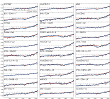
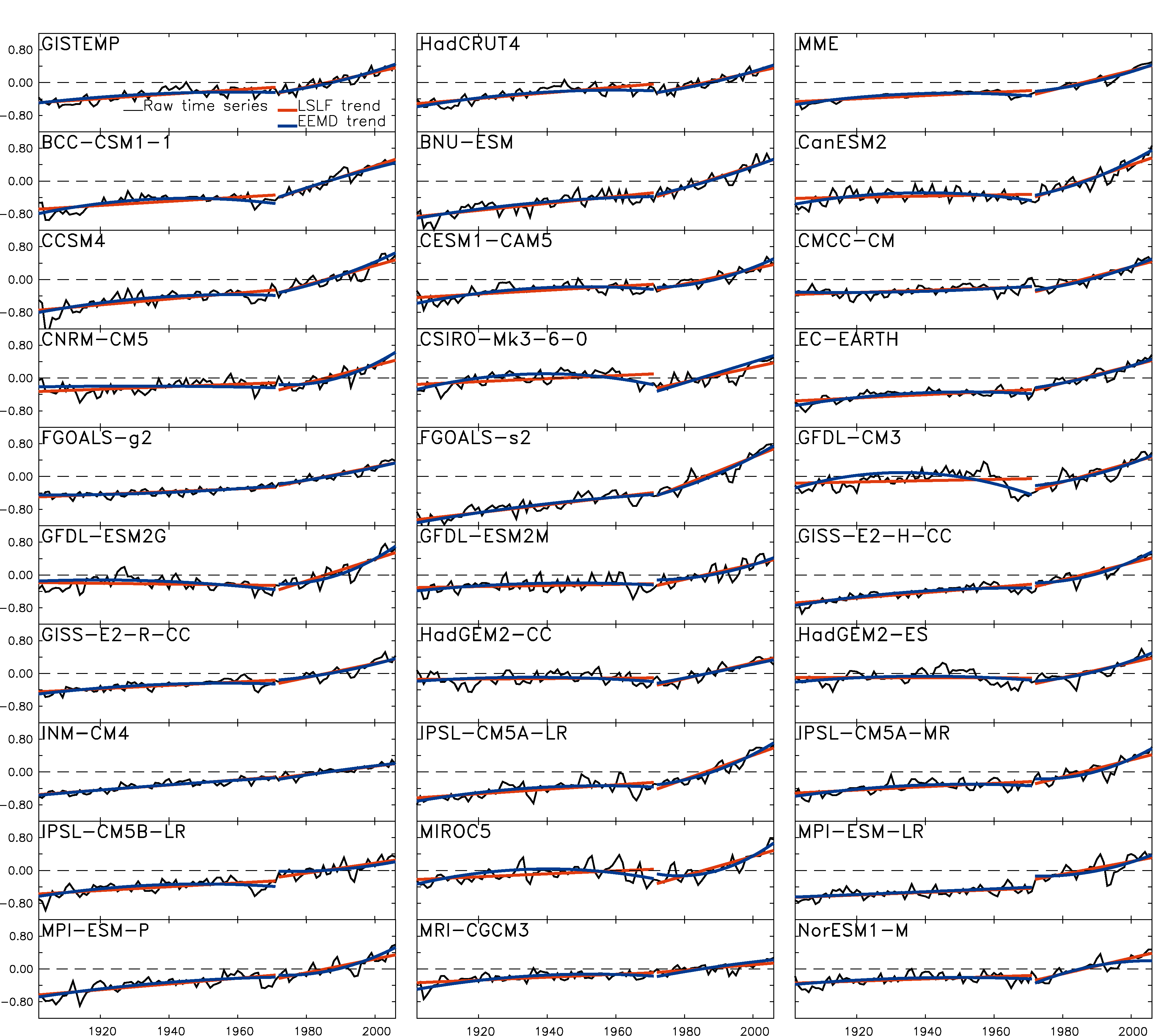
The observed global averaged SATs from GISTEMP and HadCRUT4 reveal an obvious warming signal in the 20th century (1901-2005) with a positive linear trend of 0.345° C per five decade (Fig. 1). This warming signal is composed of a slow warming from 1901 to 1970, and a rapid warming (> β 0.5° C) from 1971 to 2005. Most of the CMIP5 models capture the warming signal and its temporal features (Fig. 1), which is also presented in the time series of the (multi-model ensemble mean) MEM. The lines derived from LSLF fit the original time series for observations and simulations. However, the lines cannot capture well the upward trend in some models. The lines fitted by the EEMD trend with the addition of the multi-decadal variability (MDV) component can reproduce the original time series much better than the lines only derived from the EEMD trend component. During the period of 1901-2005, the trend values of the EEMD trend with the addition of the MDV component are larger than those of LSLF trends in most of the models (Table 2).

Figure 1

Figure Option ViewDownloadNew Window

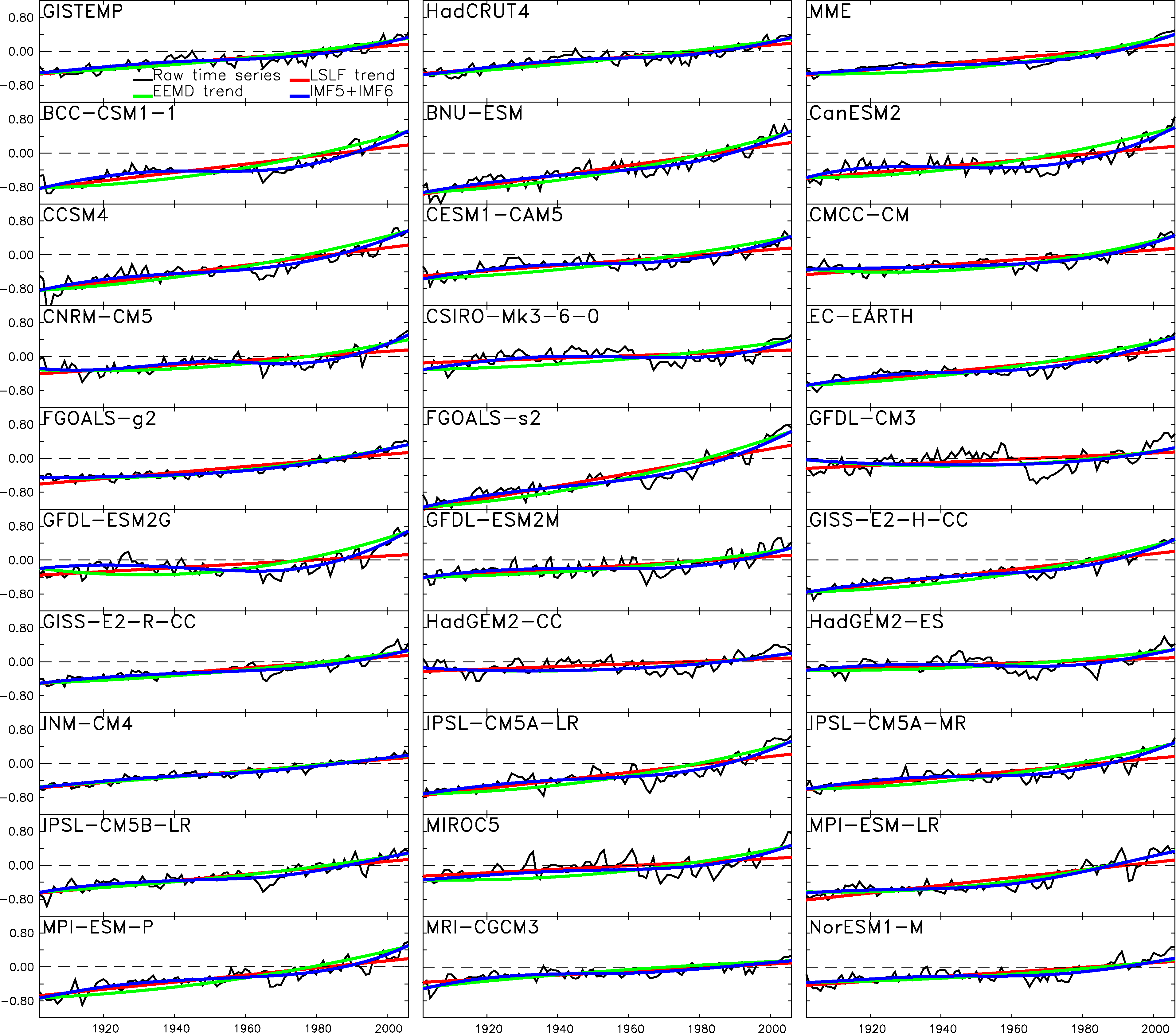Figure 1 Time series (black curves) of global averaged surface air temperature (SAT) (° C) annual mean anomalies (relative to 1971-2000) and their lines fitted by the Least Squares Linear Fitting (LSLF) (red curves), by the Ensemble Empirical Mode Decomposition (EEMD) trend component (green curves), and by EEMD multi-decadal variability and trend components (blue curves) during the period 1901-2005 in observations from the National Aeronautics and Space Administration Goddard Institute for Space Studies Surface Temperature Analysis (GISTEMP) and the Met Office Hadley Centre and Climatic Research Unit latest version (HadCRUT4), 27 individual models, and the multi-model ensemble (MME).

Table 2

Table 2

Table 2 Trend values (° C per five decade) calculated by LSLF and EEMD approaches. MEM is the multi-member ensemble mean. Models Period and trend 1901-2005 1901-70 1971-2005 LSLF trend EEMD trend + MDV LSLF trend EEMD trend LSLF trend EEMD trend GISTEMP 0.34 0.4 0.27 0.18 0.9 0.97 HadCRUT4 0.345 0.42 0.35 0.28 0.89 0.95 MEM 0.345 0.445 0.2 0.15 1.03 0.92 BCC-CSM1-1 0.49 0.645 0.25 0.18 1.396 1.2 BNU-ESM 0.585 0.69 0.42 0.38 1.32 1.23 CanESM2 0.365 0.565 0.07 0.06 1.4 1.57 CCSM4 0.515 0.67 0.36 0.3 1.18 1.39 CESM1-CAM5 0.315 0.48 0.23 0.24 0.91 0.99 CMCC-CM 0.295 0.38 0.13 0.1 1.08 1.08 CNRM-CM5 0.27 0.38 0.15 -0.02 1.06 1.12 CSIRO-Mk3-6-0 0.145 0.33 0.19 0.08 0.9 1.24 EC-EARTH 0.405 0.54 0.2 0.2 1.05 0.99 FGOALS-g2 0.355 0.37 0.17 0.16 0.82 0.74 FGOALS-s2 0.73 0.855 0.48 0.49 1.68 1.71 GFDL-CM3 0.185 0.135 0.08 -0.12 1.18 1.05 GFDL-ESM2G 0.23 0.42 -0.05 -0.15 1.33 1.31 GFDL-ESM2M 0.255 0.335 0.07 0.1 0.92 0.77 GISS-E2-H-CC 0.465 0.59 0.33 0.3 1.03 1.08 GISS-E2-R-CC 0.32 0.37 0.21 0.17 0.87 0.74 HadGEM2-CC 0.155 0.165 0.03 -0.01 0.97 0.82 HadGEM2-ES 0.14 0.235 -0.01 0.03 0.91 0.98 INM-CM4 0.345 0.36 0.31 0.3 0.51 0.55 IPSL-CM5A-LR 0.47 0.595 0.27 0.25 1.47 1.45 IPSL-CM5A-MR 0.38 0.52 0.2 0.18 1.04 1.06 IPSL-CM5B-LR 0.38 0.445 0.23 0.17 0.61 0.33 MIROC5 0.21 0.39 0.18 0.09 1.19 1.07 MPI-ESM-LR 0.455 0.47 0.14 0.17 0.78 0.73 MPI-ESM-P 0.42 0.59 0.35 0.34 0.84 0.96 MRI-CGCM3 0.22 0.315 0.18 0.23 0.33 0.58 NorESM1-M 0.27 0.275 0.14 0.09 0.97 0.78

Table 2 Trend values (° C per five decade) calculated by LSLF and EEMD approaches. MEM is the multi-member ensemble mean.

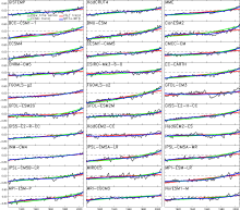
To examine the possible differences in the trend line during the slow and rapid warming periods by these two approaches, the fitted lines in these two periods are displayed in Fig. 2. During the slow warming period (1901-70), the lines by the EEMD trend component fit the original time series better than those by LSLF. Meanwhile, the trends by LSLF are larger than those by EEMD in observations and most of the models in this period (Table 2). During the rapid warming period (1971-2005), the lines by the EEMD trend component also fit the original time series better than those by LSLF, although the trends by LSLF are comparable with those by EEMD in observations and most of the models. In some models (FGOALS-g2, INM-CM4, CMCC-CM), the lines reconstructed by LSLF and EEMD fit very well, suggesting the trends are mainly linear in these models.

Figure 2

	Figure Option ViewDownloadNew Window
	Figure 2 Time series (black curves) of global averaged SAT (° C) annual mean anomalies (relative to 1971-2000) and their lines fitted by LSLF (red curves) and by the EEMD trend component (blue curves) during the periods of 1901-70 and 1971-2005 in observations from GISTEMP and HadCRUT4, 27 individual models, and the MME.

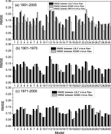
Figure 3 shows the RMSEs between reconstructed lines (LSLF, EEMD trend component or EEMD trend + IMF5 components, IMF5 representing MDV component, ~ 60 yr) and the original time series during 1901-2005. About half of the models have larger RMSEs between the reconstructed lines by the EEMD trend component and the original time series compared with that between the reconstructed lines by LSLF and the original time series. When the reconstructed lines include the EEMD MDV and trend components, smaller RMSE is obtained in most of the models compared with that by the reconstructed lines by LSLF during 1901-2005. This implies the MDV is important for estimating the temporally varying trend during the period of 1901-2005, which has been pointed out in some previous studies (e.g., Wu et al., 2011).

Figure 3

Figure Option ViewDownloadNew Window

Figure 3 RMSEs (° C) between raw time series (or lines) and the fitted lines of global averaged SAT anomalies during the periods of (a) 1901-2005, (b) 1901-70, and (c) 1971-2005. The x-axes are labeled with the 27 model numbers; the MME is shown in the 28th column; and the observed trends from GISTEMP and HadCRUT4 are shown in the 29th and 30th columns, respectively. Black bars: lines fitted by LSLF minus Raw; gray bars: lines fitted by the EEMD trend minus Raw; white bars: lines fitted by EEMD MDV and trend components minus Raw.

RMSEs are calculated during the slow and rapid warming periods by splitting the whole period (1901- 2005) based on these two approaches. Smaller RMSEs are achieved in most of the models during these two shorter periods for the reconstructed lines only by the EEMD trend component by comparing those reconstructed straight lines for LSLF. Such a short length of time is not necessary to add the other component, except for the EEMD trend component to the reconstruction of the lines for fitting the original time series because the effect of MDV cannot be removed from the EEMD trend component (e.g., Ji et al., 2014). This also suggests it is better to estimate the trend using EEMD than LSLF especially for short time periods with obvious nonlinear behavior.

According to the above comparison, EEMD is a good choice to extract the trend (or global warming rate). In Table 2, the warming rates by the two approaches are given. During the period of 1901-2005, the trend values by EEMD trend + MDV components are larger (smaller) in 12 (10) models (total: 27) than those from observations. Among 12 (10) models, the larger (smaller) trend values also exist in 9 (8) models during the rapid warming period. This means for most of the models, if they have higher (lower) sensitivity to greenhouse gases (e.g., CO₂), the trends (global warming rates) will be larger (smaller) during 1901-2005. During the slow warming period, 6 (5) models among 12 (10) models also have larger (smaller) trends than those from observations. This implies a high (low) sensitivity to greenhouse gases exists in the 6 (5) models for both the slow and rapid warming periods. This low and high sensitivity will lead to the smaller and larger global warming rates during the period of 1901-2005.

On a global scale, the EEMD trends are slightly lower than the LSLF trends over the slow warming period. The EEMD approach extracts the overall trend from the different time scales’ internal variability. As is known, trends would be affected by sampling fluctuations of internal variability (Feldstein, 2002; Franzke, 2009), and the role of internal variability in global warming is potentially important, especially before the 1970s (e.g., Deser et al., 2012). Besides, the slight cooling from 1940-70 can be captured by the EEMD approach. Therefore, the EEMD trend can better reflect the slow warming before the 1970s because the LSLF approach cannot capture the internal variability at different time scales and in several cooling years. For an anthropogenic-caused trend during the rapid warming period, the EEMD approach is also demonstrated to be a powerful approach for extracting true trends.

In this study, we use EEMD and LSLF to estimate the historical SAT trends in 27 CMIP5 models and observations from GISTEMP and HadCRUT4 during the period 1901-2005. We also examine the trends using these approaches during the slow and rapid warming periods. The magnitudes of the trends estimated by the two approaches are comparable. The trend calculated by the EEMD approach is larger than that by the LSLF approach in most of the models (23/27) during 1901-2005. The RMSEs between the raw time series and the reconstructed one by the LSLF approach are slightly smaller than that by the EEMD trend component, but larger than that by the EEMD trend and MDV components during 1901-2005 in most of the models and observations. This implies the MDV is important for estimating the temporally varying trend during the period 1901-2005. During the slow warming period, the EEMD trend is smaller than the LSLF trend. During 1901-70 (or 1971-2005), the RMSEs between the raw time series and the reconstructed one by LSLF are larger than those by the EEMD trend component. In this sense, the EEMD trend is a better choice to obtain the climate trends in observations and CMIP5 models, especially for short time periods. For short time periods (< β 70 yr), the trend and MDV (~ 60 yr) are not clearly separated by EEMD IMFs. The LSLF approach cannot capture the SAT change during the slow warming period. This is because the LSLF cannot capture the internal variability for such short slow warming periods.

By comparing the trends by EEMD in different periods, we find the estimated global warming rates (trend) are larger (smaller) than those from observations during 1901-2005 for 11 of 27 models if the response to greenhouse gases (e.g., CO₂) are higher (lower) during both the slow and rapid warming periods. EEMD can extract the signals at different time scales, and the trends. Using this approach, we can compare the trend and internal variability at different time scales and provide insight regarding the attribution and detection of global warming.