

Optimal Precursor Perturbations of El Niño in the Zebiak-Cane Model for Different Cost Functions
Cite this Article
XU Hui. Optimal Precursor Perturbations of El Niño in the Zebiak-Cane Model for Different Cost Functions. Atmospheric and Oceanic Science Letters, 2014, 7(4): 297-303 
Permissions
Copyright?2014, Editorial office of Atmospheric and Oceanic Science Letters
This is an Open Access article under the terms of CCAL.
Optimal Precursor Perturbations of El Niño in the Zebiak-Cane Model for Different Cost Functions
Abstract
Optimal precursor perturbations of El Niño in the Zebiak-Cane model were explored for three different cost functions. For the different characteristics of the eas-tern-Pacific (EP) El Niño and the central-Pacific (CP) El Niño, three cost functions were defined as the sea surface temperature anomaly (SSTA) evolutions at prediction time in the whole tropical Pacific, the Niño3 area, and the Niño4 area. For all three cost functions, there were two optimal precursors that developed into El Niño events, called Precursor I and Precursor II. For Precursor I, the SSTA component consisted of an east-west (positive-neg-ative) dipole spanning the entire tropical Pacific basin and the thermocline depth anomaly pattern exhibited a tendency of deepening for the whole of the equatorial Pacific. Precursor I can develop into an EP-El Niño event, with the warmest SSTA occurring in the eastern tropical Pacific or into a mixed El Niño event that has features between EP-El Niño and CP-El Niño events. For Precursor II, the thermocline deepened anomalously in the eastern equatorial Pacific and the amplitude of deepening was obviously larger than that of shoaling in the central and western equatorial Pacific. Precursor II developed into a mixed El Niño event. Both the thermocline depth and wind anomaly played important roles in the development of Precursor I and Precursor II.
Keyword:
El Niño; CNOP; optimal precursor; cost function
1 Introduction
El Niño-Southern Oscillation (ENSO) is a coupled ocean-atmosphere phenomenon in the tropical Pacific and has received much attention for both its climatic and economic effects. It has been increasingly recognized that two different types of El Niño occur in the tropical Pacific based on the spatial distributions of the SST: the eastern-Pacific (EP) El Niño and the central-Pacific (CP) El Niño ( Ashok et al., 2007; Kao and Yu, 2009; Kug et al., 2009). EP-El Niño events show a stronger warm SST ano-maly in the eastern tropical Pacific and extend to the central tropical Pacific. The Niño3 SSTA (sea surface temperature anomaly) is an appropriate index to measure the intensity of EP-El Niño events ( Rasmusson and Carpenter, 1982). Unlike EP-El Niño events, CP-El Niño events have warm SST anomalies in the central Pacific, especially near the International Date Line ( Larkin and Harrison, 2005). The Niño4 SSTA is an appropriate index to measure the intensity of CP-El Niño events. Some events have features between EP- and CP-El Niño events. The maximum SST anomalies of these eve-nts are located between 120°W and 150°W and Kug et al. (2009) called them "mixed El Niño events".
Numerous models have been developed to simulate and predict ENSO events ( Battisti and Hirst, 1989; Kleeman, 1993; Jin, 1997a, b; Rosati et al., 1997; Wang et al., 1999). Although significant achievements have been made, notable differences between models and reality still rem-ain. Moreover, CP-El Niño events became more common during the late twentieth century, especially after the 1990s, which has increased the challenge for many models to predict ENSO events ( Kug et al., 2010; Kim et al., 2012).
Identifying the precursors for ENSO is of great significance for improving ENSO predictability ( Duan et al., 2004). Many studies have used the linear singular vector (LSV) method and attempted to find out the initial pattern that is most likely to evolve into an ENSO event, i.e., the optimal precursor for ENSO ( Blumenthal, 1991; Kleeman, 1993; Moore and Kleeman, 1996; Thompson, 1998). However, the linear theory of singular vector always supposes that the evolution of the initial perturbation can be described approximately by the linearized version, i.e., tangent linear model (TLM) of the nonlinear model. Then, because of the absence of nonlinearity, the fastest growing initial perturbation in TLM could not be the optimal perturbation in the nonlinear model ( Oortwijin and Barkmeijier, 1995; Mu and Wang, 2001).
Considering the limitation of the LSV method, Mu et al. (2003) proposed a novel concept of conditional non-linear optimal perturbation (CNOP), which is characterized by the maximum nonlinear growth of the initial perturbation in a given constraint condition and has been app-lied to study the optimal precursor of ENSO. Xu (2006) applied the CNOP method to the Zebiak-Cane (ZC) model ( Zebiak and Cane, 1987) and investigated the optimal precursor of ENSO. Duan et al. (2008) studied the decisive role of nonlinear temperature advection in the El Niño and La Niña amplitude asymmetry. Mu et al. (2013) further proposed the similarities between optimal precursors for ENSO events and optimally growing initial errors in El Niño predictions. Duan et al. (2013) investigated the behaviors of nonlinearities modulating the El Niño events induced by optimal precursor disturbances.
For the above studies, the optimal precursor of El Niño always developed into an EP-El Niño event in the ZC model, which is quite different from the observations that there are not only EP-El Niño but also CP-El Niño events. But what causes this phenomenon? We noticed that the cost functions in their studies were all designed as the development of SSTA in the whole tropical Pacific at the prediction time. Because the intensity of observed EP-El Niño is usually stronger than that of observed CP-El Niño, naturally, we ask: does the defined cost function make it inevitable that the ZC model finds the precursor of EP-El Niño? And can the precursor of CP-El Niño be found by defining other appropriate cost functions?
This study aims to answer the above questions. By defining different cost functions, we used the CNOP appro-ach to explore the optimal precursors of El Niño events in the ZC model. The paper is organized as follows. In section 2, the ZC model is briefly described and the concept of CNOP is presented. In section 3, we show the numerical results of the optimal precursors for El Niño events by defining different cost functions. Section 4 interprets the developing mechanism of optimal precursors. Finally, we present a discussion and the conclusions in section 5.
2 The ZC model and CNOP method
The ZC model was the first coupled ocean-atmosphere model to simulate the interannual variability of the observed ENSO. It has since been widely used in predictability studies and the prediction of ENSO ( Cane et al., 1986; Zebiak and Cane, 1987; Xue et al., 1994; Chen et al., 1995, 2004). The ZC model depicts the thermodynamics and atmospheric dynamics in the tropical Pacific. The corresponding equations govern the evolution of oceanic and atmospheric perturbations superimposed on a specified climatological annual cycle.
The ZC atmospheric model is defined in the region on a 2° latitude × 5.625° longitude grid with latitude from 29°S to 29°N and longitude from 101.25°E to 73.125°W. The region on a 0.5° latitude × 2° longitude grid of ZC oceanic dynamics extends from 28.75°S to 28.75°N and from 124°E to 80°W. The SSTA equation describes the evolution of temperature anomalies in the model surface layer and the SSTA is computed in the region on a 2° latitude × 5.625° longitude grid with latitude from 19°S to 19°N and longitude from 129.375°W to 84.375°W. For more details of the ZC model, see Zebiak and Cane (1987).
The CNOP approach is a natural generalization of the LSV approach to nonlinear systems. Let
For a chosen norm,
| (1) |
where
To compute the CNOP, we need to solve Eq. (1). However, Eq. (1) is a maximization problem, and there is currently no method to directly calculate it. So, Eq. (1) was transformed into a minimization problem by considering the reciprocal of the cost function
| (2) |
The CNOP can be solved using the following minimum problem:
| (3) |
The first variation of
| , (4) |
where the operation
3 Optimal precursors of El Niño events for different cost functions
3.1 Design of numerical experiments
Considering the different characteristics of EP-El Niño and CP-El Niño, we constructed three cost functions related to the CNOP, which were defined as the SSTA development at prediction time in the whole tropical Pacific (19°S-19°N, 129.375°E-84.375°W), in the Niño3 area (5°S-5°N, 150°-90°W), and in the Niño4 area (5°S-5°N, 160°E-150°W). Then, the CNOP approach was used to investigate the optimal precursors of two types of El Niño events in the ZC model.
The ZC model is an anomalous model with respect to the climatological annual cycle, and the cost functions can be written as follows:
| (5) |
where
We then computed the CNOPs in the ZC model. For the optimization periods
3.2 Precursors for different cost functions
Numerical results showed that when the cost function was defined as the SSTA development in the whole tropical Pacific and in the Niño3 area, the CNOP always cau-sed a warm event and the local CNOP always caused a cold event in the tropical Pacific. Comparing the patterns of CNOP and SSTA development after 12 months of both cost functions, they were very similar for each initial month. Due to the length of the paper, we focus on the results of the latter.
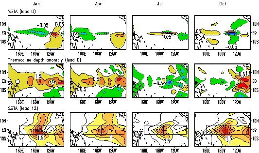
Figure 1 shows the pattern of optimal precursor and SSTA development after 12 months when the cost function was defined in the Niño3 area, for different initial months. We can see that when the initial SSTA pattern consisted of an east-west (positive-negative) dipole spanning the entire tropical Pacific basin and the thermocline depth anomaly pattern exhibited a tendency of deepening for the whole of the equatorial Pacific, the nonlinear evolution of the CNOP made the eastern and central tropical Pacific extremely warm after 12 months. The SSTA max-imums after 12 months were uniformly located in the Niño3 area for the initial months of January, April, July, and October, which illustrates that all these CNOPs developed into EP-El Niño events and so it can be considered the optimal precursor of EP-El Niño events.
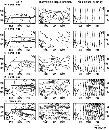
Figure 2 shows the pattern of optimal precursor and SSTA development after 12 months when the cost function was defined in the Niño4 area. We can see that, for this cost function, all precursors for the different initial months made the central Pacific extremely warm and the eastern Pacific warm, and developed into the mixed El Niño events mentioned by Kug et al. (2009). The warmest center of SSTA was located near 150°W and 30° west of the location for the cost function in the Niño3 area.
However, the precursors for the different initial months in Fig. 2 are quite different from those in Fig. 1. Comparing Fig. 2 with Fig. 1, we can see that the pattern of precursor for the initial months of January and April is somewhat similar to those in Fig. 1. For the initial month of July, the pattern of precursor is almost contrary to those for the cost function in the Niño3 area. In fact, the precursor of El Niño for the initial month of July in Fig. 3 is somewhat similar to the precursor that develops to a La Niña event when the cost function is defined in the Niño3 area (figure omitted). For the initial month of October, the pattern of precursor is quite different from those for the other initial months, and the initial positive thermocline depth anomaly in the eastern equatorial Pacific is a distinct feature.
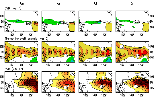 | Figure 1 Optimal precursors and the sea surface temperature anomaly (SSTA) after 12 months with the initial months being January, April, July, and October for the cost function defined as the SSTA development in the Niño3 area. The top panels are the initial SSTA component, the middle panels are the initial thermocline depth anomaly component, and the bottom panels are the SSTA development after 12 months. The square frames label the Niño3 and Niño4 areas. |
 | Figure 2 Optimal precursors and the sea surface temperature anomaly (SSTA) after 12 months with the initial months being January, April, July, and October for the cost function defined as the SSTA development in the Niño4 area. The top panels are the initial SSTA component, the middle panels are the initial thermocline depth anomaly component, and the bottom panels are the SSTA development after 12 months. The square frames label the Niño3 and Niño4 areas. |
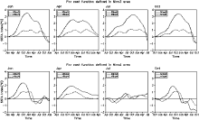
Figure 3 shows the two-year developments of the Niño3 and Niño4 indices during the period that the optimal pre-cursors developed into El Niño events. We can see that, when the cost function was defined as the Niño3 SSTA, the peak of the Niño3 index of the El Niño event caused by the precursor occurred in the winter of the year for the initial months of January and April, and occurred in the winter of the next year for the initial months of July and December. That is to say, regardless of the initial month, the EP-El Niño events caused by the optimal precursors phase-lock to winter, which agrees with the features of the observed El Niño events.
For the cost function defined in the Niño4 area, the two-year developments of the Niño3 and Niño4 indices during the period that the optimal precursors develop to El Niño events are also shown in Fig. 3. We can see that the peaks of the Niño3 or Niño4 indices of these El Niño events do not occur uniformly in winter. That is, these mixed El Niño events caused by the optimal precursors fail to phase-lock to winter. Moreover, the precursor for the initial month of July developed toward a cold phase in the first months and then developed toward to a warm phase.
The above results show that when the cost function was defined as the SSTA in the whole tropical Pacific or the Niño3 area, we found quite similar optimal precursors that developed to EP-El Niño events regardless of the optimization period and initial month. When the cost function was defined as the Niño4 SSTA, the optimal precursors developed to mixed El Niño events, but the patterns of these precursors were different. In the following, we explore the developing mechanism of these precursors.
4 Developing mechanism of optimal precursors
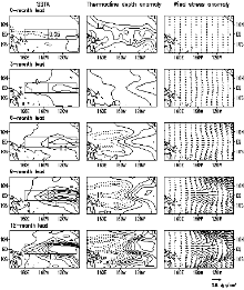
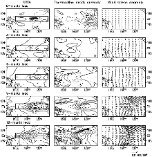
For the initial month of October, there were two different precursors for the cost functions defined in the Niño3 and Niño4 areas. We called them Precursor I and Precursor II. We then used these precursors as initial fields for the ZC model and investigated the developments of atmospheric and oceanic states (shown in Figs. 4 and 5).
In Fig. 4, the pattern of Precursor I is characterized by an east-west (positive-negative) dipole spanning the entire tropical Pacific basin and a deepening of the equatorial thermocline. Because the thermocline in the eastern equatorial Pacific was very close to the surface, there was a natural tendency to produce a positive SSTA that was largest in the east. This positive SSTA was superimposed on the existing positive SSTA. The atmospheric response, an equatorial westerly wind anomaly in the center tropical Pacific, was then established. The influence of the westerly wind anomaly deepened the eastern ocean thermocline, suppressing the equatorial upwelling, and setting up the eastward current anomalies, all of which tended to reinforce the SSTA in the center and eastern tropical Pacific. Thus, the Bjerknes (1969) positive warm feedback explains the evolution of the CNOP.
In Fig. 5, for Precursor II, the thermocline deepens anomalously in the eastern equatorial Pacific and the amplitude of deepening is obviously larger than that of shoaling in the central and western equation Pacific. From a 0-month to 3-month lead, the positive thermocline depth anomaly caused a warm SSTA in the eastern tropical Pacific and the original negative SSTA in the eastern equatorial Pacific developed to some extent but moved west, which led to an westerly wind anomaly in the eastern pacific and a easterly wind anomaly in the central Pacific. From a 3-month to 6-month lead, though the thermocline depth anomaly was faintly negative, the wind anomaly played a relatively important role in the development of the SSTA. The westerly wind anomaly increased gradually in the central Pacific and made the SSTA warmer by anomalous zonal advection. From a 6-month to 12-month lead, the joint effect of the westerly wind anomaly in the central tropical Pacific and the easterly wind anomaly in the eastern tropical Pacific made the location of the warmest SSTA move westward. Both the wind anomaly and the thermocline deepened in the eastern and central Pacific to help the warmest SSTA occur in the central Pacific and Precursor II developed to a mixed El Niño event.
 | Figure 3 The time series of the Niño3 and Niño4 index. The top (bottom) panels corresponds to the cost function defined as the SSTA in the Niño3 (Nino4) area. The solid line is the Niño3 index and the dashed line is the Niño4 index. |
 | Figure 4 The evolution patterns of the optimal precursor with initial time (October) and lead times 3, 6, 9, and 12 months for the cost function defined as the SSTA development in the Niño3 area. The left column is the SSTA component, the middle column is the thermocline depth anomaly component, and the right column is the corresponding wind stress anomalies. The square frames label the Niño3 and Niño4 areas. The contour interval is 0.05°C for 0-month lead SSTA, 0.5°C for other SSTA, 0.5 m for 0-month lead thermocline depth anomaly, and 5.0 m for others. |
For the initial months of January and April, the pattern of the precursor when the cost function defined in Niño4 area was similar to Precursor I, but developed to a mixed El Niño event. Comparing their developing processes, we can see that the different locations of the easterly wind, westerly wind, and the largest thermocline depth anomaly led to a different location of the warmest SSTA.
5 Discussion and conclusions
The CNOP method was used in the ZC model to find the optimal precursor perturbations of El Niño events. Considering the different characteristics of EP-El Niño and CP-El Niño, we constructed three cost functions, which were defined as the SSTA evolution in the whole of the tropical Pacific, the Niño3 area, and the Niño4 area. For all three cost functions, there were two optimal precursors that developed into El Niño events-Precursor I and Precursor II. For Precursor I, the SSTA component consisted of an east-west (positive-negative) dipole spanning the entire tropical Pacific basin and the thermocline depth anomaly pattern exhibited a tendency of deepening over the whole of the equatorial Pacific. Precursor I can develop into an EP-El Niño event with the warmest SSTA occurring in the eastern tropical Pacific or into a mixed El Niño event with the warmest SSTA located near 150°W. For Precursor II, the thermocline deepened anomalously in the eastern equatorial Pacific and the amplitude of deepening was obviously larger than that of shoaling in the central and western equation Pacific. Precursor II developed into a mixed El Niño event. Both the thermocline depth and wind anomaly played important roles in the development of Precursor I and Precursor II.
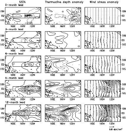 | Figure 5 The evolution patterns of the optimal precursor with initial time (October) and lead times 3, 6, 9, and 12 months for the cost function defined as the SSTA development in the Niño4 area. The left column is the SSTA component, the middle column is the thermocline depth anomaly component, and the right column is the corresponding wind stress anomalies. The square frames label the Niño3 and Niño4 areas. The contour interval is 0.05°C for 0-month lead SSTA, 0.5°C for other SSTA, 0.5 m for 0-month lead thermocline depth anomaly, and 5.0 m for others. |
Precursor I caused the warmest SSTA to be located in the eastern tropical Pacific or near 150°W and then caused different effects on the global climate, which added difficulties to ENSO prediction. These results imply that if we improve the data in the sensitive equatorial Pacific by target observations we may improve the prediction of ENSO.
In this study, for three different cost functions, we fai-led to find the optimal precursor that develops into a CP- El Niño event, which may imply that the ZC model has no ability to give a good simulation for CP-El Niño. In the future, we will conduct numerical experiments to simulate observed CP-El Niño events by a four-dimensional variability assimilation method and explore whether the ZC model has a good ability to simulate CP-El Niño.
Acknowledgments. The author thanks Dr. Stephen E. ZEBIAK for providing the ZC model. This work was jointly supported by the National Natural Science Foundation of China (Grant No. 41006007) and the National Basic Research Program of China (Grant No. 2012CB417404).
Reference
| 1 |
|
| 2 |
|
| 3 |
|
| 4 |
|
| 5 |
|
| 6 |
|
| 7 |
|
| 8 |
|
| 9 |
|
| 10 |
|
| 11 |
|
| 12 |
|
| 13 |
|
| 14 |
|
| 15 |
|
| 16 |
|
| 17 |
|
| 18 |
|
| 19 |
|
| 20 |
|
| 21 |
|
| 22 |
|
| 23 |
|
| 24 |
|
| 25 |
|
| 26 |
|
| 27 |
|
| 28 |
|
| 29 |
|
| 30 |
|
| 31 |
|
| 32 |
|
| 33 |
|